Call:
lm(formula = Mass_g ~ condition, data = demo)

Coefficients:
  (Intercept)  conditiontest
       1147.6         -105.1
Call:
lm(formula = Mass_g ~ tank, data = demo)

Coefficients:
(Intercept)    tanktank2
1147.6 -105.1 Bio300B Lecture 10
Institutt for biovitenskap, UiB
19 October 2025
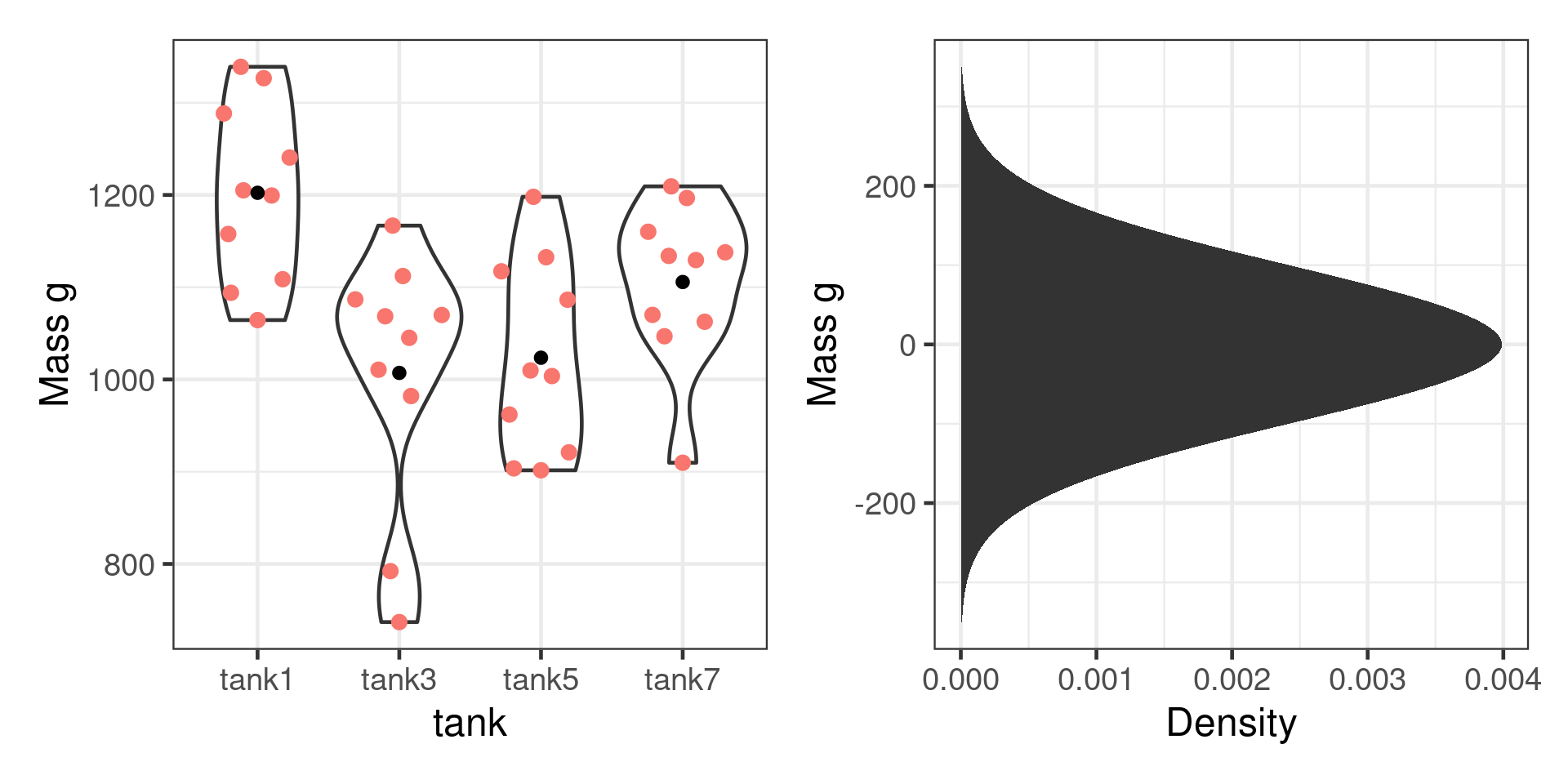
Observations not independent
Ignoring it causes pseudoreplication
True effect of treatment: 100 g
Call:
lm(formula = Mass_g ~ condition, data = demo)
Coefficients:
(Intercept) conditiontest
1147.6 -105.1
Call:
lm(formula = Mass_g ~ tank, data = demo)
Coefficients:
(Intercept) tanktank2
1147.6 -105.1
Call:
lm(formula = Mass_g ~ condition + tank, data = demo2)

Residuals:
    Min      1Q  Median      3Q     Max
-270.11  -59.70   20.80   71.17  224.67

Coefficients: (1 not defined because of singularities)
              Estimate Std. Error t value Pr(>|t|)
(Intercept)    1202.37      33.38  36.021  < 2e-16 ***
conditiontest   -68.44      47.21  -1.450 0.151439
tanktank2      -118.07      47.21  -2.501 0.014654 *
tanktank3      -195.25      47.21  -4.136 9.44e-05 ***
tanktank4        33.35      47.21   0.707 0.482102
tanktank5      -178.79      47.21  -3.788 0.000313 ***
tanktank6       -49.47      47.21  -1.048 0.298128
tanktank7       -96.71      47.21  -2.049 0.044128 *
tanktank8           NA         NA      NA       NA
---
Signif. codes:  0 '***' 0.001 '**' 0.01 '*' 0.05 '.' 0.1 ' ' 1

Residual standard error: 105.6 on 72 degrees of freedom
Multiple R-squared:  0.3187,    Adjusted R-squared:  0.2525
F-statistic: 4.812 on 7 and 72 DF, p-value: 0.0001745\[y_i = \color{red}{\beta_0} + \color{red}{\beta_1}x_i + \color{red}{\beta_2}tank_i +\color{blue}{ \varepsilon_i}\]
Not interested in effect of tank
Use a Random effect
Assumes observed tanks from a population of possible tanks
\[y_{ij} = \color{red}{\beta_0} +\color{blue}{b_{0i}}+ \color{red}{\beta_1}x_i +\color{blue}{ \varepsilon_{ij}}\]
Residuals from a normal distribution \(\color{blue}{ \varepsilon_{ij}} \sim N(0, \sigma_{ind})\)
Random effects from a normal distribution \(\color{blue}{b_{0i}} \sim N(0, \sigma_{clu})\)
Linear mixed model fit by REML ['lmerMod']
Formula: Mass_g ~ condition + (1 | tank)
   Data: demo2

REML criterion at convergence: 965.8

Scaled residuals:
    Min      1Q  Median      3Q     Max
-2.6916 -0.5419  0.1989  0.6274  2.2428

Random effects:
 Groups   Name        Variance Std.Dev.
 tank     (Intercept)  5059     71.13
 Residual             11142    105.56
Number of obs: 80, groups:  tank, 8

Fixed effects:
              Estimate Std. Error t value
(Intercept)    1084.68      39.28  27.611
conditiontest    15.70      55.56   0.283

Correlation of Fixed Effects:
            (Intr)
conditintst -0.707Linear mixed model fit by REML. t-tests use Satterthwaite's method [
lmerModLmerTest]
Formula: Mass_g ~ condition + (1 | tank)
Data: demo2
REML criterion at convergence: 965.8
Scaled residuals:
Min 1Q Median 3Q Max
-2.6916 -0.5419 0.1989 0.6274 2.2428
Random effects:
Groups Name Variance Std.Dev.
tank (Intercept) 5059 71.13
Residual 11142 105.56
Number of obs: 80, groups: tank, 8
Fixed effects:
Estimate Std. Error df t value Pr(>|t|)
(Intercept) 1084.68 39.28 6.00 27.611 1.49e-07 ***
conditiontest 15.70 55.56 6.00 0.283 0.787
---
Signif. codes: 0 '***' 0.001 '**' 0.01 '*' 0.05 '.' 0.1 ' ' 1
Correlation of Fixed Effects:
(Intr)
conditintst -0.707Linear mixed-effects model fit by REML
Data: demo2
AIC BIC logLik
973.8449 983.2717 -482.9225
Random effects:
Formula: ~1 | tank
(Intercept) Residual
StdDev: 71.12618 105.555
Fixed effects: Mass_g ~ condition
Value Std.Error DF t-value p-value
(Intercept) 1084.6791 39.28460 72 27.610796 0.000
conditiontest 15.7008 55.55682 6 0.282608 0.787
Correlation:
(Intr)
conditiontest -0.707
Standardized Within-Group Residuals:
Min Q1 Med Q3 Max
-2.6916143 -0.5418500 0.1988656 0.6273686 2.2428518
Number of Observations: 80
Number of Groups: 8 glmmTMB - generalised linear mixed effect modelsbrms - Bayesian mixed effect modelsBoth use similar syntax to lme4 package
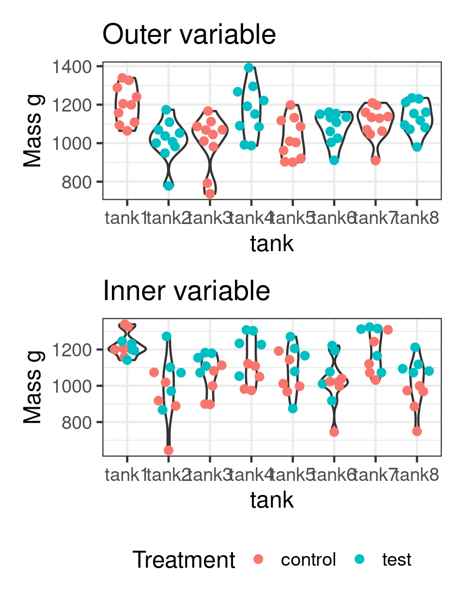
Fixed effects factors:
Random effects factors:
“one modeler’s random effect is another modeler’s fixed effect.”
“Are there enough levels of the factor in the data on which to base an estimate of the variance of the population of effects? No, means fixed effects.”
Linear mixed model fit by REML. t-tests use Satterthwaite's method [
lmerModLmerTest]
Formula: Mass_g ~ condition + (1 | tank)
   Data: demo3

REML criterion at convergence: 975.8

Scaled residuals:
     Min       1Q   Median       3Q      Max
-2.72095 -0.58452  0.09483  0.55007  1.95600

Random effects:
 Groups   Name        Variance Std.Dev.
 tank     (Intercept)  6371     79.82
 Residual             12253    110.69
Number of obs: 80, groups:  tank, 8

Fixed effects:
              Estimate Std. Error       df t value Pr(>|t|)
(Intercept)   1037.398     33.207    9.416  31.240 7.87e-11 ***
conditiontest  110.263     24.752   71.000   4.455 3.06e-05 ***
---
Signif. codes:  0 '***' 0.001 '**' 0.01 '*' 0.05 '.' 0.1 ' ' 1

Correlation of Fixed Effects:
            (Intr)
conditintst -0.373Linear mixed model fit by REML. t-tests use Satterthwaite's method [
lmerModLmerTest]
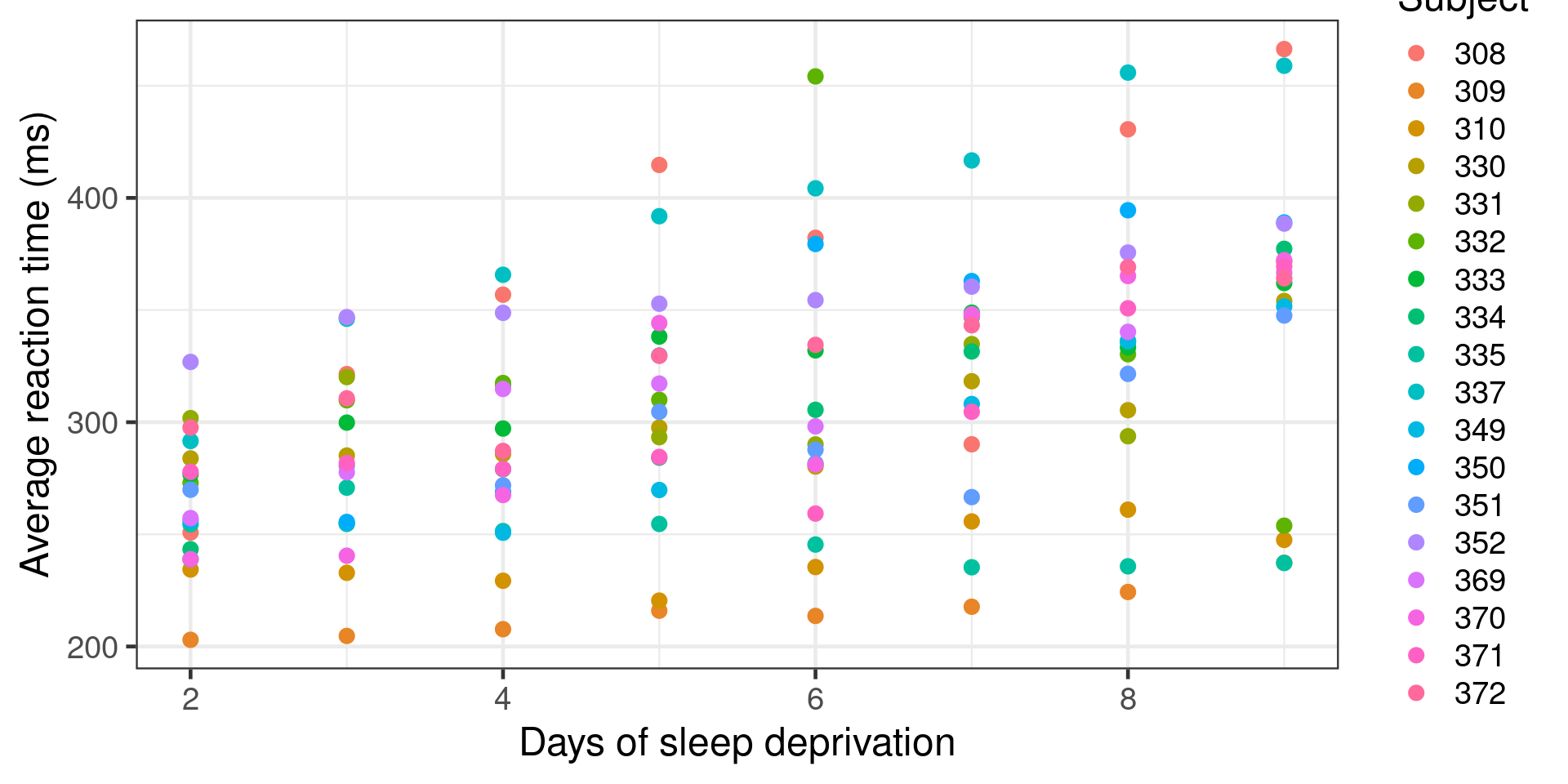
Formula: Reaction ~ Days + (1 | Subject)
Data: sleepstudy
Subset: Days >= 2
REML criterion at convergence: 1430
Scaled residuals:
Min 1Q Median 3Q Max
-3.6261 -0.4450 0.0474 0.5199 4.1378
Random effects:
Groups Name Variance Std.Dev.
Subject (Intercept) 1746.9 41.80
Residual 913.1 30.22
Number of obs: 144, groups: Subject, 18
Fixed effects:
Estimate Std. Error df t value Pr(>|t|)
(Intercept) 245.097 11.829 30.617 20.72 <2e-16 ***
Days 11.435 1.099 125.000 10.40 <2e-16 ***
---
Signif. codes: 0 '***' 0.001 '**' 0.01 '*' 0.05 '.' 0.1 ' ' 1
Correlation of Fixed Effects:
(Intr)
Days -0.511Linear mixed model fit by REML. t-tests use Satterthwaite's method [
lmerModLmerTest]
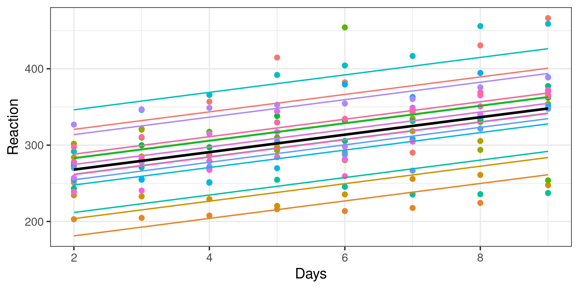
Formula: Reaction ~ Days + (Days | Subject)
Data: sleepstudy
Subset: Days >= 2
REML criterion at convergence: 1404.1
Scaled residuals:
Min 1Q Median 3Q Max
-4.0157 -0.3541 0.0069 0.4681 5.0732
Random effects:
Groups Name Variance Std.Dev. Corr
Subject (Intercept) 992.69 31.507
Days 45.77 6.766 -0.25
Residual 651.59 25.526
Number of obs: 144, groups: Subject, 18
Fixed effects:
Estimate Std. Error df t value Pr(>|t|)
(Intercept) 245.097 9.260 16.999 26.468 2.95e-15 ***
Days 11.435 1.845 17.001 6.197 9.74e-06 ***
---
Signif. codes: 0 '***' 0.001 '**' 0.01 '*' 0.05 '.' 0.1 ' ' 1
Correlation of Fixed Effects:
(Intr)
Days -0.454Data: sleepstudy
Subset: Days >= 2
Models:
fm1: Reaction ~ Days + (1 | Subject)
fm2: Reaction ~ Days + (Days | Subject)
npar AIC BIC logLik -2*log(L) Chisq Df Pr(>Chisq)
fm1 4 1446.5 1458.4 -719.25 1438.5
fm2 6 1425.2 1443.0 -706.58 1413.2 25.332 2 3.156e-06 ***
---
Signif. codes: 0 '***' 0.001 '**' 0.01 '*' 0.05 '.' 0.1 ' ' 1See ?plot.merMod
performance::check_model()
DHARMa package
Two random effects
Eggs from birds nests (first random effect - lay_nest) moved to other nests (second random effect - hatch_nest)
Hierarchical random effects
Sometimes mixed effect models report errors.
Take them seriously.
May need to simplify the model
Having predictors on same scale can help
Generalised linear mixed effect models
Fit with glmer()
Autocorrelated data
nlme::lme() or glmmTMB::glmmTMB()glmmTMB packageMixed effect models can be hard to fit
Bayesian model can help
Different statistical philosophy
rstannimbleUse prior information (or uninformative priors)
brms package fits Bayesian mixed effect models with lme4-like syntaxBolker B (2021) GLMM FAQ
Harrison et al (2018) A brief introduction to mixed effects modelling and multi-model inference in ecology