Survival analysis and Multivariate methods

Bio300B Lecture 11

Richard J. Telford (Richard.Telford@uib.no)

Institutt for biovitenskap, UiB

3 November 2026

Survival analysis

How long (or far) until an event happens

  • How long before a seed germinates
  • How long before a patient dies after diagnosis
  • How many jumps can a horse clear at a racecourse

Data are typically right censored.

survival package

Survival data

Response data

  • time
  • status (alive/dead coded as 0/1, 1/2 TRUE/FALSE)
library(survival)
lung |> slice(1:10)
   inst time status age sex ph.ecog ph.karno pat.karno meal.cal wt.loss
1     3  306      2  74   1       1       90       100     1175      NA
2     3  455      2  68   1       0       90        90     1225      15
3     3 1010      1  56   1       0       90        90       NA      15
4     5  210      2  57   1       1       90        60     1150      11
5     1  883      2  60   1       0      100        90       NA       0
6    12 1022      1  74   1       1       50        80      513       0
7     7  310      2  68   2       2       70        60      384      10
8    11  361      2  71   2       2       60        80      538       1
9     1  218      2  53   1       1       70        80      825      16
10    7  166      2  61   1       2       70        70      271      34

Survival response

+ indicates censored data

Surv(lung$time, lung$status)
 [1]  306   455  1010+  210   883  1022+  310   361   218   166   170   654 
[13]  728    71   567   144   613   707    61    88   301    81   624   371 
[25]  394   520   574   118   390    12 

Fitting a model

lung <- lung |> 
  mutate(sex = factor(sex, levels = 1:2, labels = c("male", "female")))

mod_surv <- survfit(Surv(time, status) ~ sex, data = lung)

mod_surv
Call: survfit(formula = Surv(time, status) ~ sex, data = lung)

             n events median 0.95LCL 0.95UCL
sex=male   138    112    270     212     310
sex=female  90     53    426     348     550

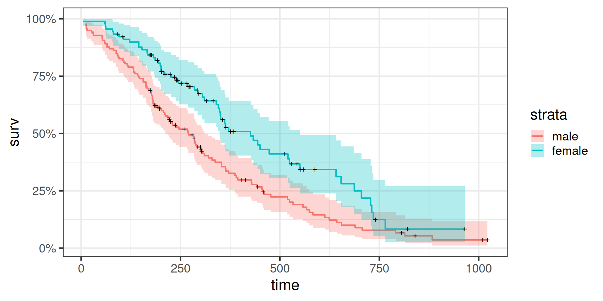
Plotting a model

  • Kaplan-Meier curve
  • ‘+’ mark censored data
library(ggfortify)
autoplot(mod_surv)

Testing differences in survival time

  • between two or more groups
mod_diff <- survdiff(Surv(time, status) ~ sex, data = lung)
mod_diff
Call:
survdiff(formula = Surv(time, status) ~ sex, data = lung)

             N Observed Expected (O-E)^2/E (O-E)^2/V
sex=male   138      112     91.6      4.55      10.3
sex=female  90       53     73.4      5.68      10.3

 Chisq= 10.3  on 1 degrees of freedom, p= 0.001 

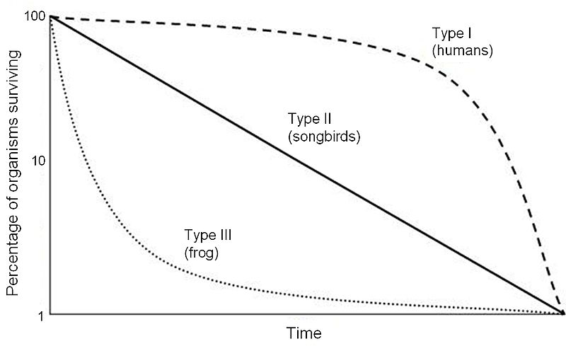
Survivorship curve

Shape of the survival curve

Hazard: The instantaneous risk of death

m_ll <- survreg(Surv(time, status) ~ age + sex, 
                data = lung,
                dist = "loglogistic")
summary(m_ll)

Call:
survreg(formula = Surv(time, status) ~ age + sex, data = lung, 
    dist = "loglogistic")
               Value Std. Error     z       p
(Intercept)  6.39982    0.49256 12.99 < 2e-16
age         -0.01401    0.00771 -1.82 0.06946
sexfemale    0.47751    0.14036  3.40 0.00067
Log(scale)  -0.56991    0.06543 -8.71 < 2e-16

Scale= 0.566 

Log logistic distribution
Loglik(model)= -1152.9   Loglik(intercept only)= -1160.9
    Chisq= 16.07 on 2 degrees of freedom, p= 0.00032 
Number of Newton-Raphson Iterations: 4 
n= 228 

Exponentiated coefficients show relative increase or decrease in the expected survival times when a covariate is increased one step while others are fixed:

exp(coef(m_ll))
(Intercept)         age   sexfemale 
601.7394821   0.9860925   1.6120541 

Expected survival time decreases by 1.4 % (i.e. multiply by 0.986) for each additional year of age

Expected survival time for females is 61.2 % higher than for males (multiply by 1.612).

scale

m_ll$scale
[1] 0.5655786

The scale parameter < 1, indicates that slope of the hazard decreases with time - Type III

Choice of distribution

Distribution df
exponential 1
Weibull 2
lognormal 2
log logistic 2

Can use AIC to choose best

m_w <- update(m_ll, dist = "weibull")
AIC(m_ll, m_w)
     df      AIC
m_ll  4 2313.794
m_w   4 2302.109

Mixed effect survival analysis

Survival of nestlings in nests

  • nest is a random effect

coxme package

library(coxme)
fit <- coxme(Surv(time, status) ~ ph.ecog + age + (1|inst), data = lung)
fit
Cox mixed-effects model fit by maximum likelihood
  Data: lung
  events, n = 163, 226 (2 observations deleted due to missingness)
  Iterations= 18 75 
                   NULL Integrated    Fitted
Log-likelihood -739.375  -729.7294 -727.0504

                  Chisq   df          p   AIC  BIC
Integrated loglik 19.29 3.00 2.3800e-04 13.29 4.01
 Penalized loglik 24.65 4.48 9.7942e-05 15.69 1.83

Model:  Surv(time, status) ~ ph.ecog + age + (1 | inst) 
Fixed coefficients
              coef exp(coef)    se(coef)    z       p
ph.ecog 0.47319522  1.605115 0.119179189 3.97 7.2e-05
age     0.01139445  1.011460 0.009430508 1.21 2.3e-01

Random effects
 Group Variable  Std Dev    Variance  
 inst  Intercept 0.14695545 0.02159591
Multivariate data

All methods so far - single response variable

Multivariate statistics - multiple response variable

  • plant species abundances
  • physical & chemical measurements
  • climate data

Ordinations, cluster analysis

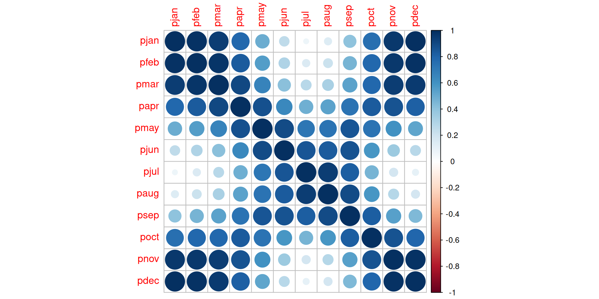
Correlation matrices

library(analogue)
library(corrplot)
data("Climate")
ppt <- Climate |> select(pjan:pdec)
mat <- cor(ppt)
corrplot(mat) # also try GGally::ggpairs

Ordinations

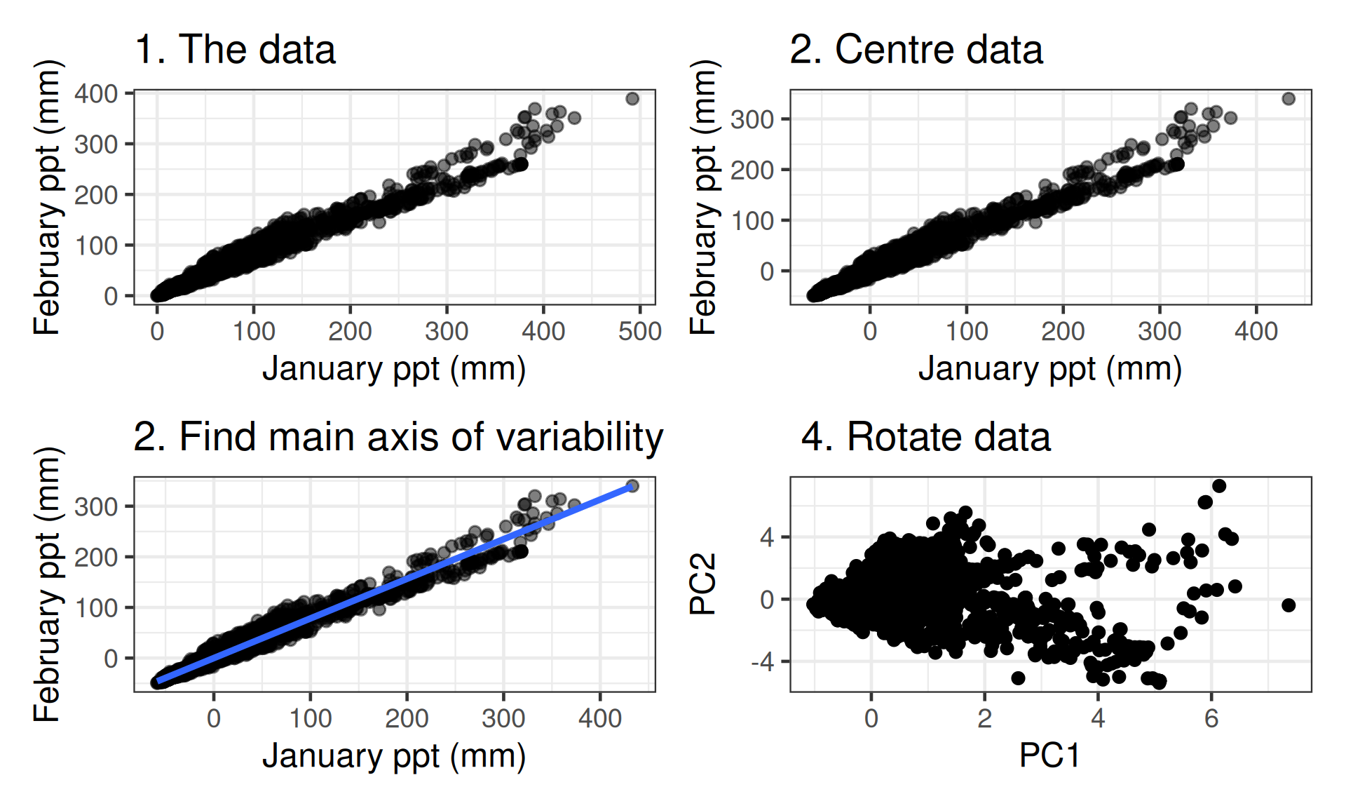
  • make sense of multivariate data by focusing on main axes of variability
  • separate signal from noise

Several methods appropriate for different types of data

  • principal components analysis
  • correspondence analysis
  • non-metric multidimensional scaling

Principal components analysis

Principal components analysis in R

Implemented in several packages

library(vegan)
pca <- rda(ppt)
pca

Call: rda(X = ppt)

              Inertia Rank
Total           29114     
Unconstrained   29114   12

Inertia is variance

Eigenvalues for unconstrained axes:
  PC1   PC2   PC3   PC4   PC5   PC6   PC7   PC8   PC9  PC10  PC11  PC12 
21534  5967   698   415   218    97    65    34    30    25    17    14 

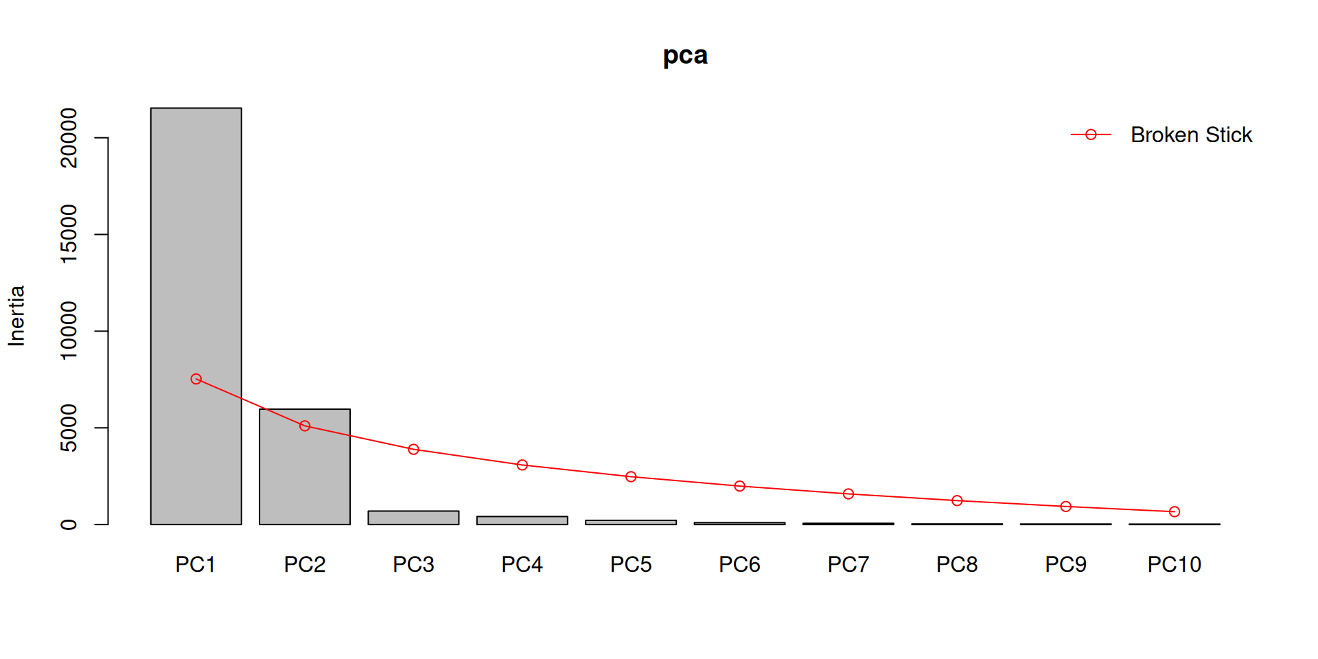
Screeplots

  • Show length of each eigenvector
  • Can help decide how many axes to interpret
  • Can use broken stick null model to help decide
screeplot(pca, bstick = TRUE)

Plotting the PCA

# plot(pca) # can make prettier
library(ggvegan) #remotes::install_github("gavinsimpson/ggvegan")
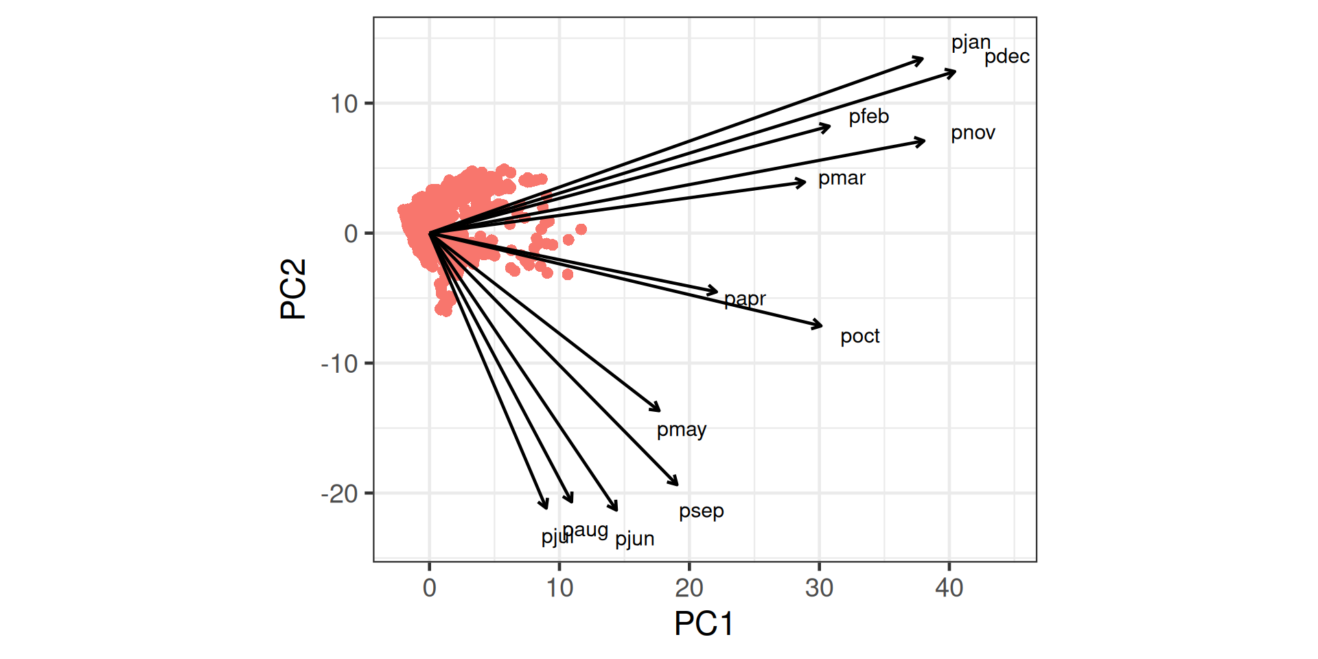
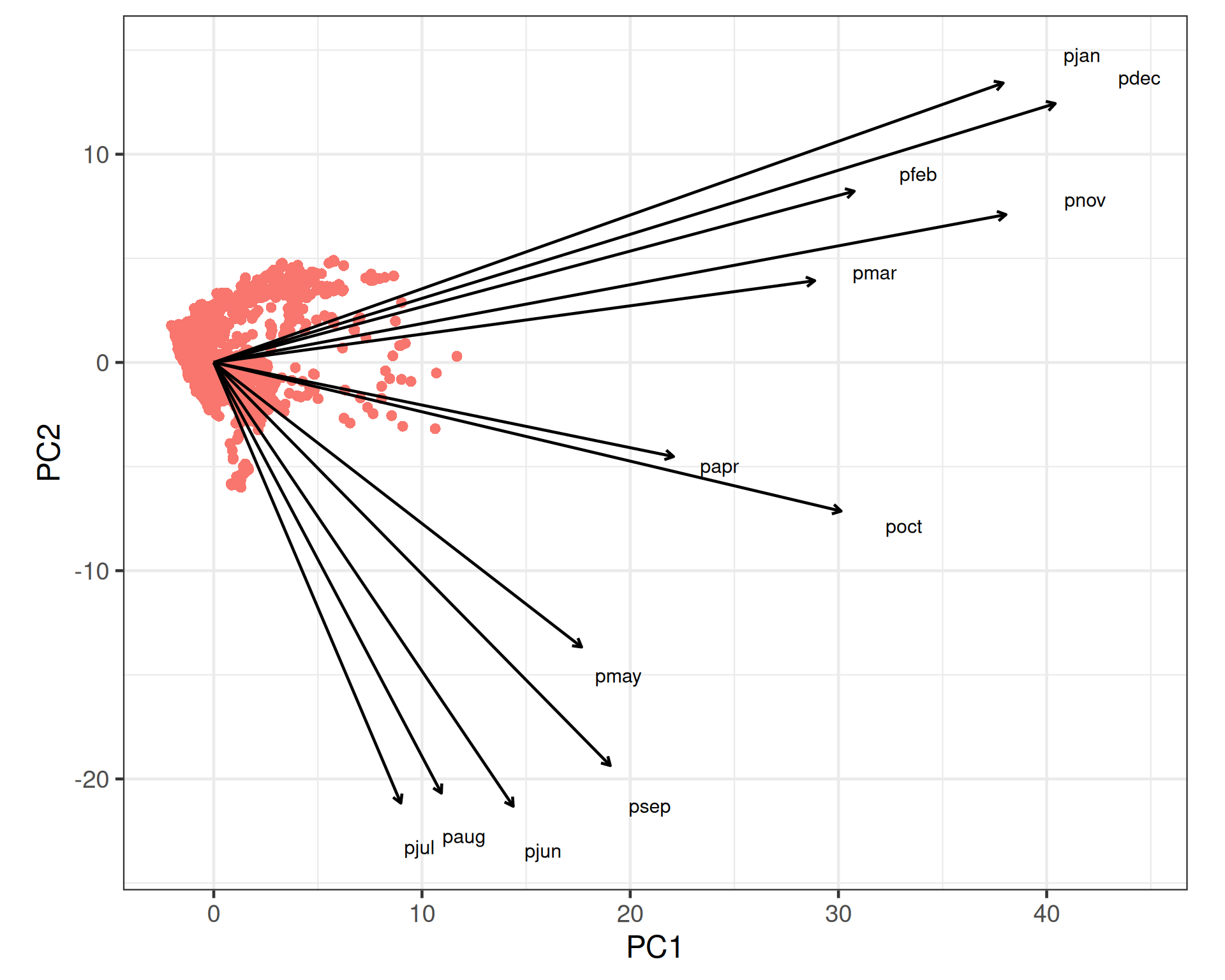
autoplot(pca) + theme(legend.position = "none")

Interpreting the plot

  • dots are observations (sites)
  • dots close together are similar
  • arrows are variables
  • arrows point in direction of increasing values
  • arrows close together are correlated
  • arrow length shows importance on axes shown

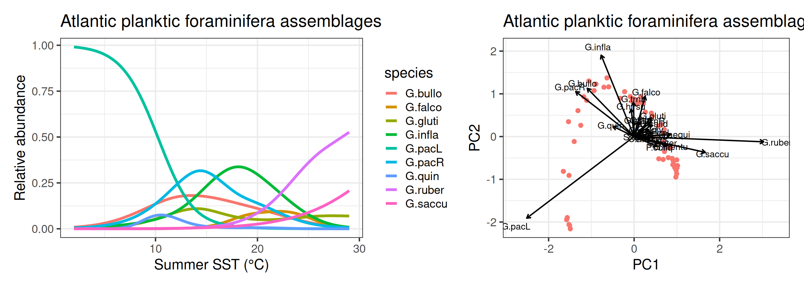
Artefacts

  • PCA assumes linear relationships between variables
  • valid for environmental data; fails for species data with long gradients