Non-linear analyses and summary

Bio300B Lecture 12

Richard J. Telford (Richard.Telford@uib.no)

Institutt for biovitenskap, UiB

3 November 2026

Assumptions of Least Squares

  1. Linear relationship between response and predictors.
  2. The residuals have a mean of zero.
  3. The residuals have constant variance (not heteroscedastic).
  4. The residuals are independent (uncorrelated).
  5. The residuals are normally distributed.

Not all relationships are linear.

Non-linear least squares can be used when relationship is non-linear.

Non-linear least squares

We know something about
the relationship

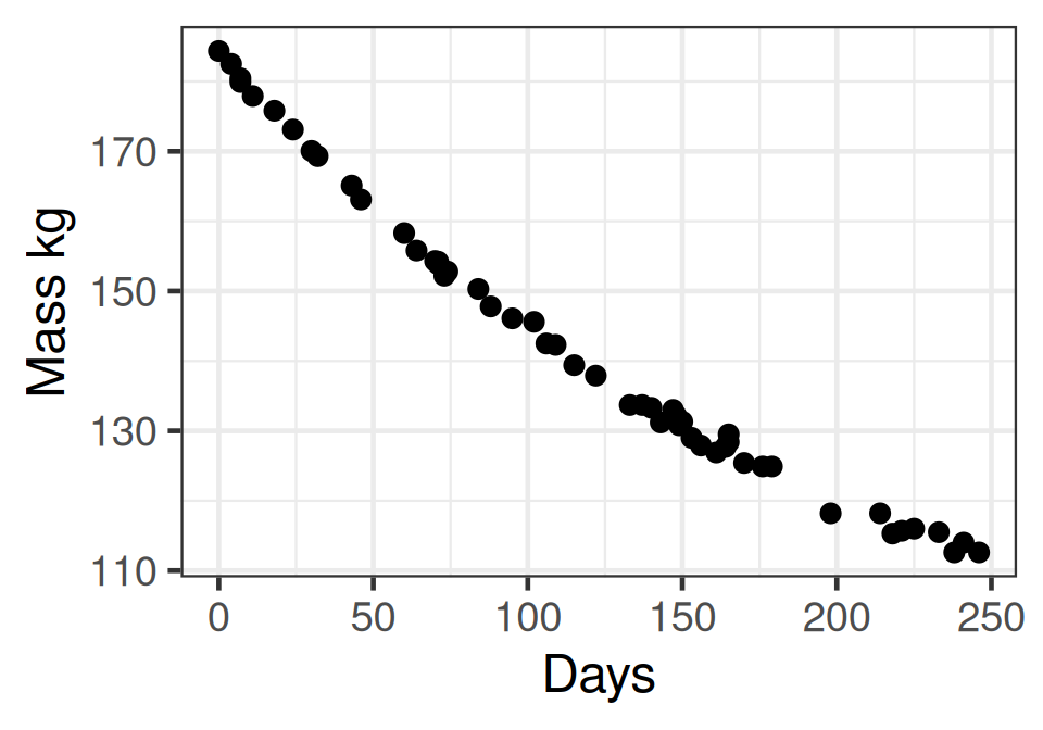
Mass of a dieting patient - has lower bound - asymptote.

Three options

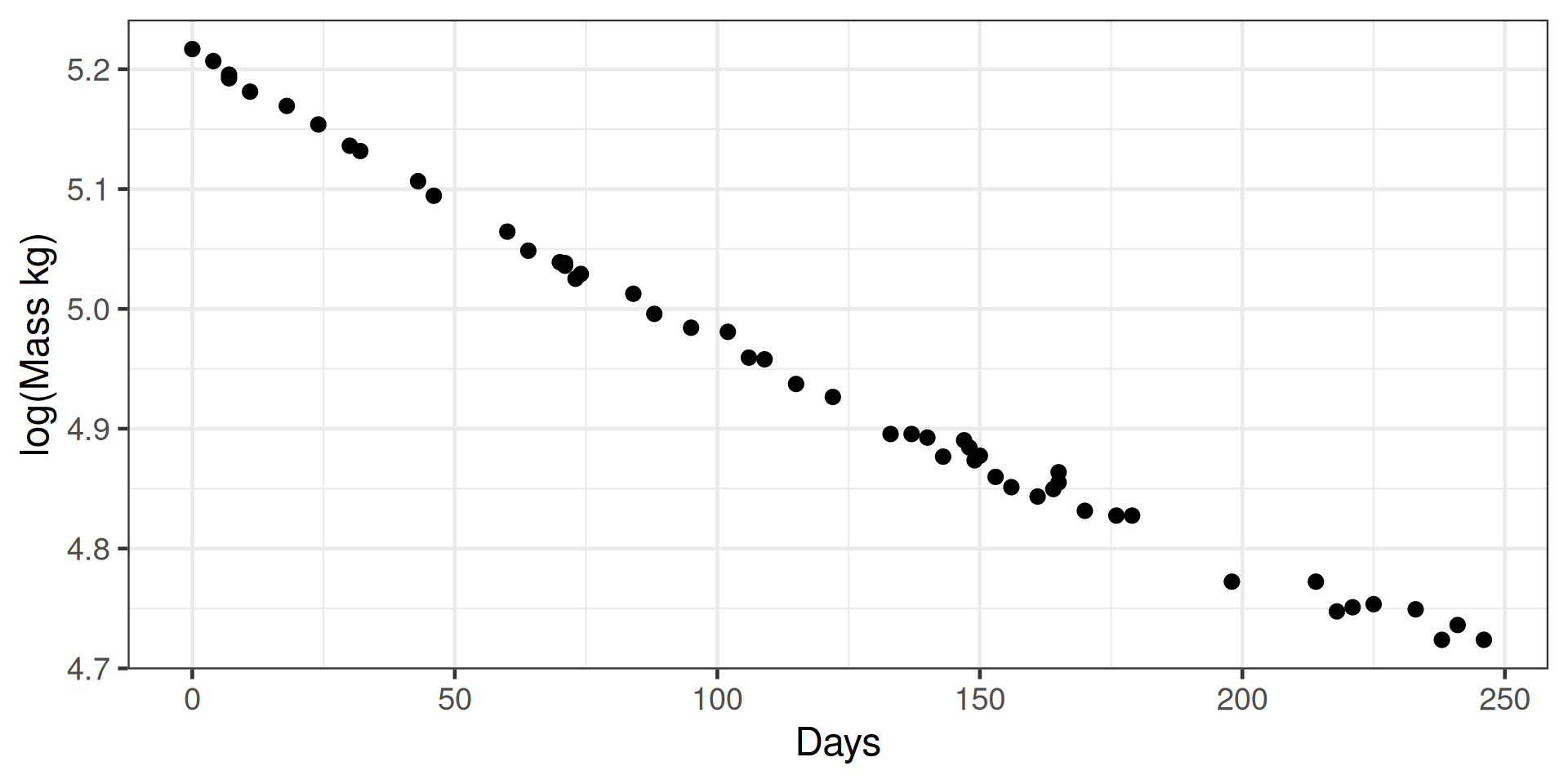
  • Transform response
  • Use polynomials (\(x^2\))
  • Non-linear expression

Transformations

  • statistics must be correct on transformed scale
  • Log transform assumes that error is a constant proportion of the response - valid for lognormal distribution
  • check diagnostics

Polynomial

\[y_i=\beta_0 + \beta_1x_i+\beta_2x^2 + \varepsilon_i\]

  • Very useful
  • Can give incorrect predictions
  • Orthogonal polynomials with poly()

Non-linear least squares

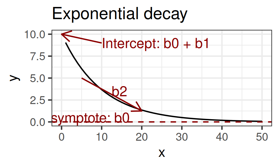
The relationship has an asymptote, and a exponential decline

\(y_i = \beta_0 + \beta_1\exp(\beta_2x_i) + \varepsilon_i\)
If \(\beta_2 < 0\)

limit \(x\to\infty\)

  • \(\beta_1\exp(\beta_2x_i) = 0\)

limit \(x\to0\)

  • \(\beta_1\exp(\beta_2x_i) = β_1\)

  • \(\beta_0\) = asymptote
  • \(\beta_0 + \beta_1\) = intercept
  • \(\beta_2\) = slope (proportional change)

Fitting an NLS

library(nlme)

fit.nls <- nls(Weight ~ b0 + b1 * exp(b2 * Days), data = wtloss)
Error in `getInitial.default()`:
! no 'getInitial' method found for "function" objects

Needs stating values - initial estimates of the coefficients

Estimating starting values

\(y_i = \beta_0 + \beta_1\exp(\beta_2x_i) + \varepsilon_i\)

  • \(\beta_0\) = asymptote
  • \(\beta_0 + \beta_1\) = intercept
  • \(\beta_2\) = slope (proportional change)

With starting values

fit.nls <- nls(Weight ~ b0 + b1 * exp(b2 * Days), 
               data = wtloss, 
               start = c(b0 = 100, b1 = 70, b2 = -0.1))
summary(fit.nls)

Formula: Weight ~ b0 + b1 * exp(b2 * Days)

Parameters:
     Estimate Std. Error t value Pr(>|t|)    
b0  8.137e+01  2.269e+00   35.86   <2e-16 ***
b1  1.027e+02  2.083e+00   49.30   <2e-16 ***
b2 -4.884e-03  1.822e-04  -26.80   <2e-16 ***
---
Signif. codes:  0 '***' 0.001 '**' 0.01 '*' 0.05 '.' 0.1 ' ' 1

Residual standard error: 0.8949 on 49 degrees of freedom

Number of iterations to convergence: 7 
Achieved convergence tolerance: 1.763e-07

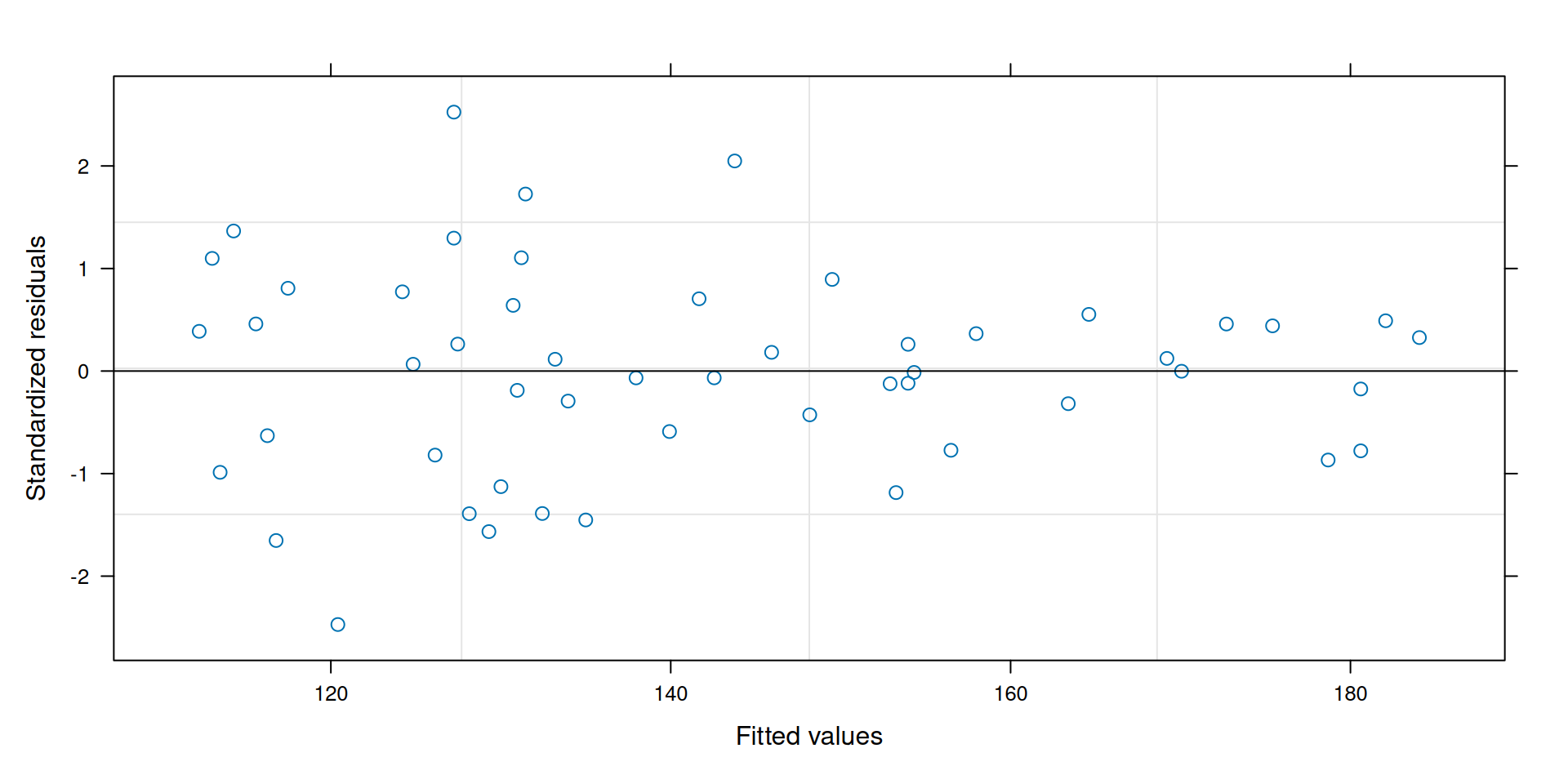
Model diagnostics

plot(fit.nls)

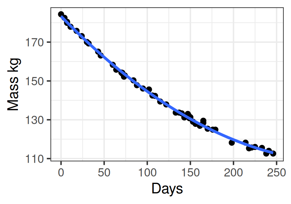
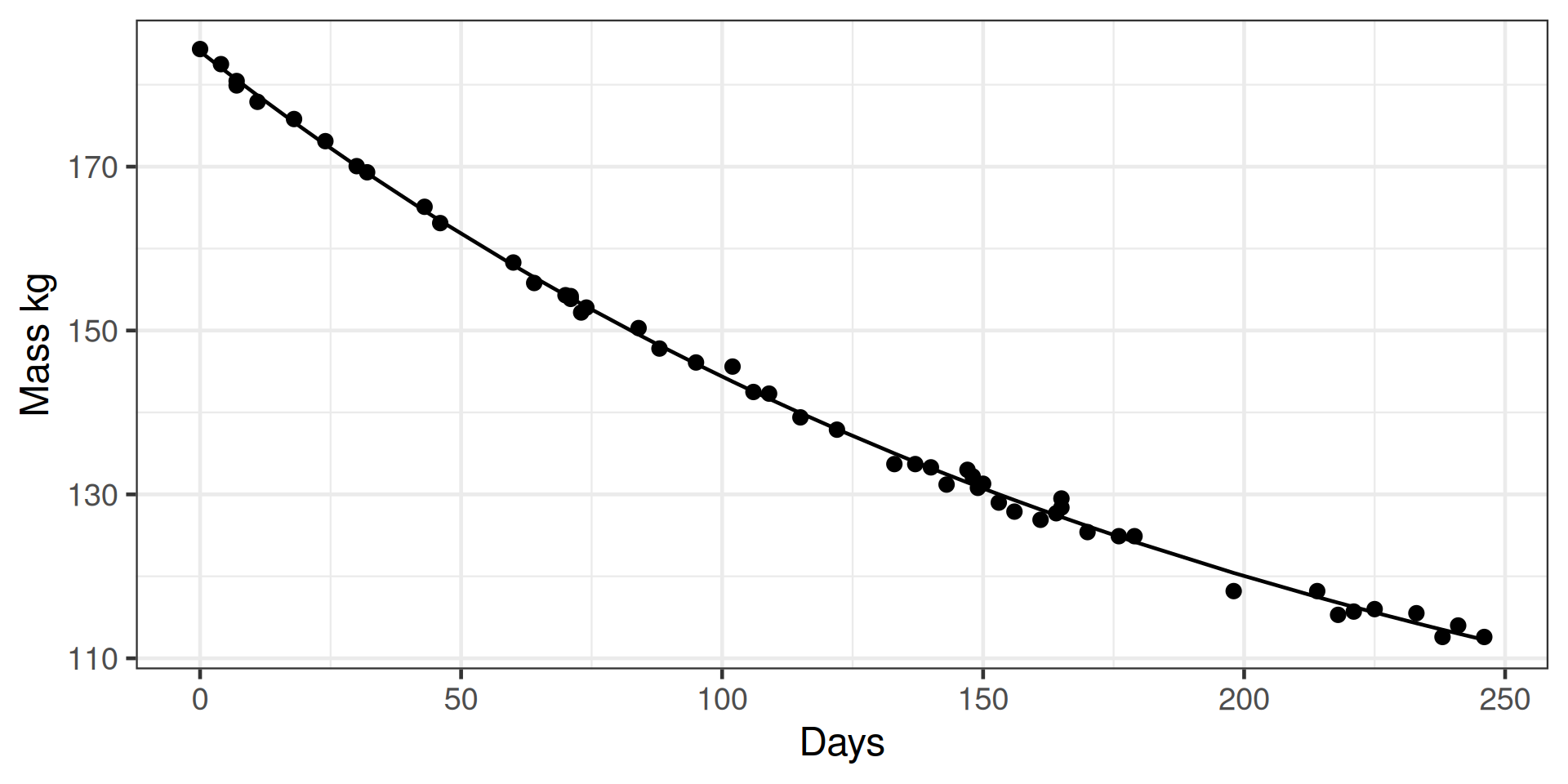
Plotting the model

p +  geom_line(data = broom::augment(fit.nls), aes(y = .fitted))

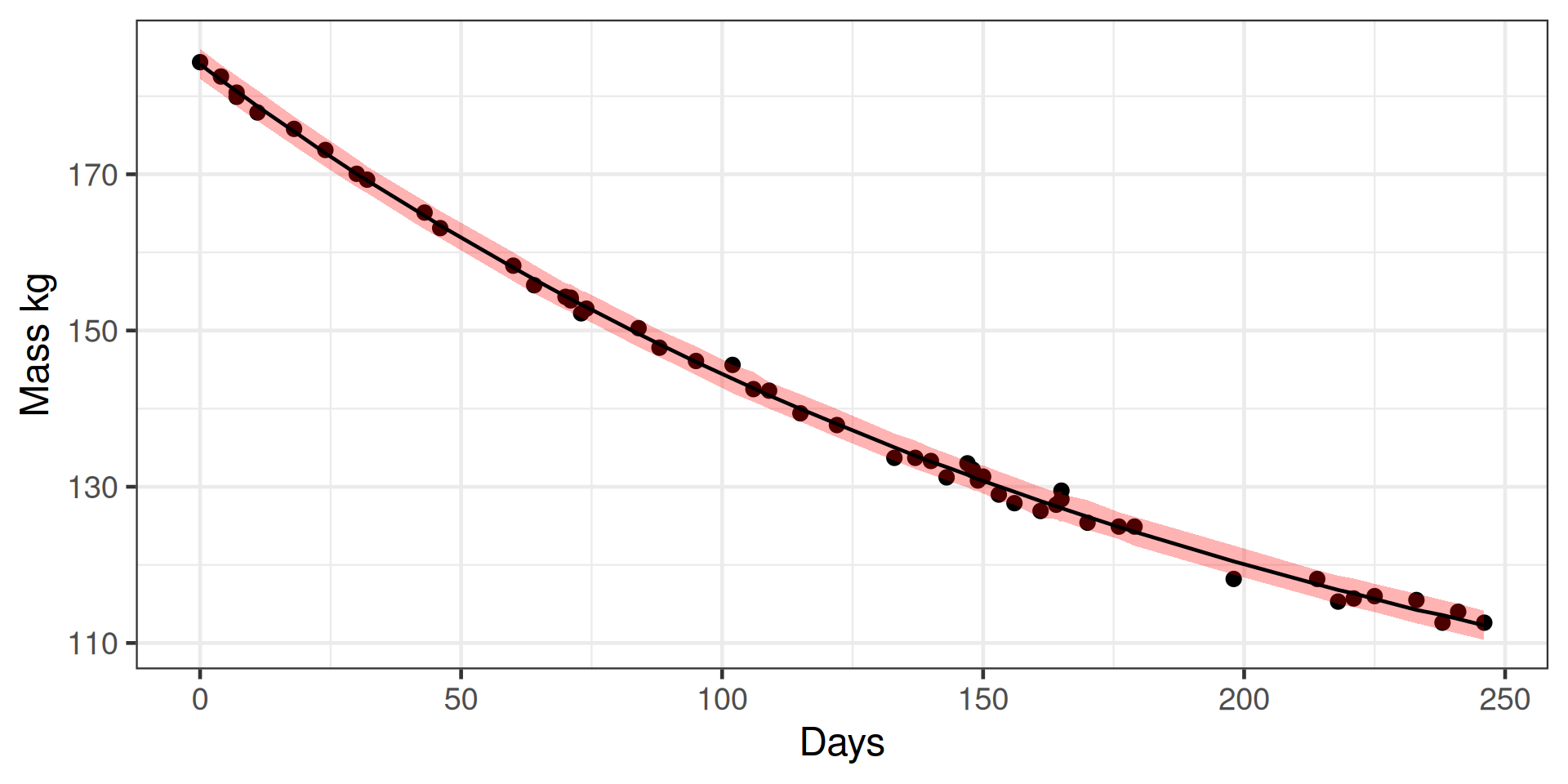
Uncertainty on model predictions

Not calculated by the model - use bootstrap

library(nlstools)
fit.boot <- nlsBoot(fit.nls)
pred <- nlsBootPredict(fit.boot, interval = "prediction") |> 
  bind_cols(wtloss)

p + geom_ribbon(aes(ymin = `2.5%`, ymax = `97.5%`), data = pred, alpha = 0.3, fill = "red") +
  geom_line(aes(y = Median), data = pred)

Working with NLS

  1. Is there a natural expression
  2. Identify parameters
  3. Roughly estimate parameters
  4. Start NLS

Example NLS models

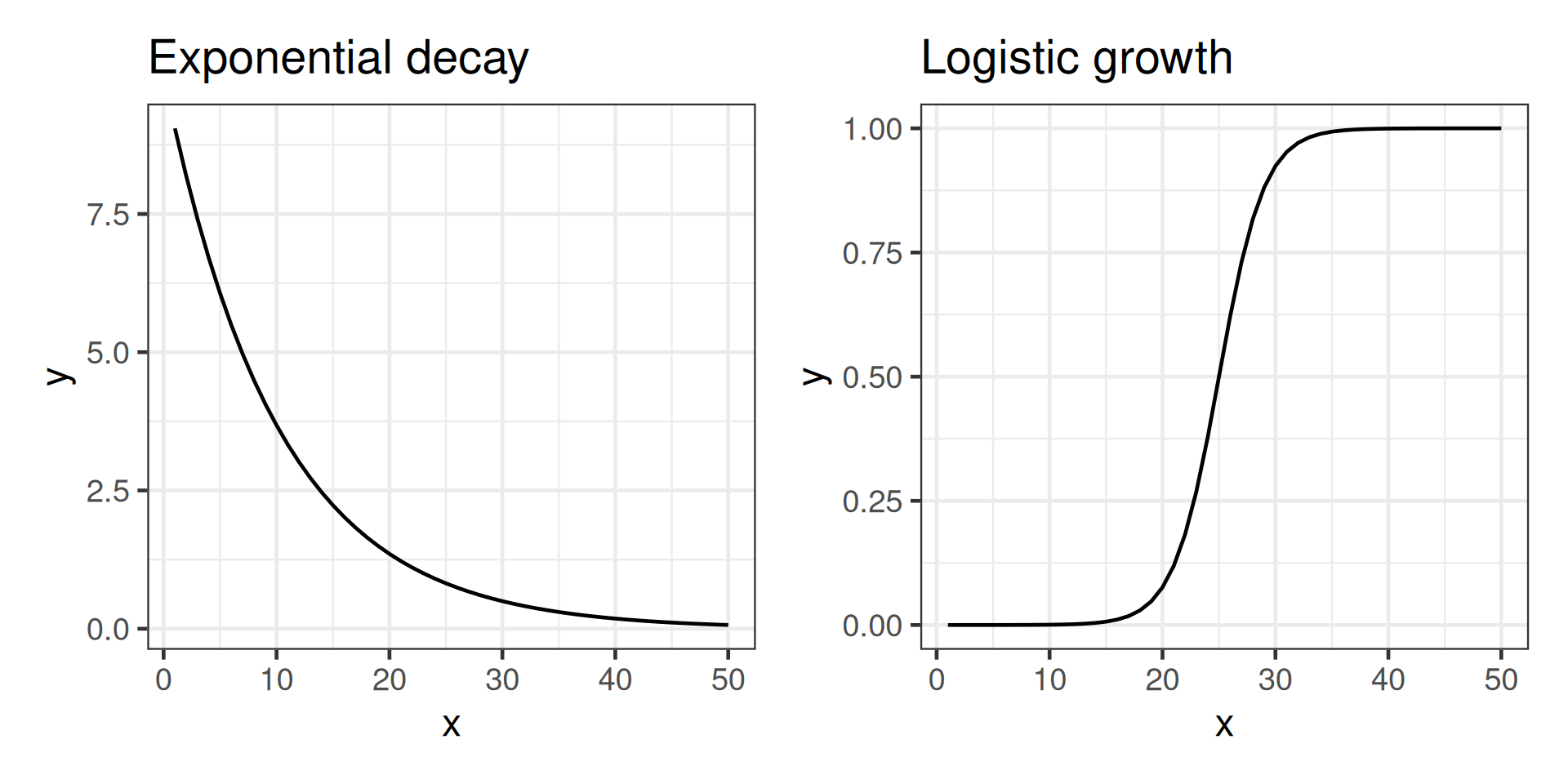
  • Exponential decay
  • Logistic growth
  • Von Bertalanffy and Gompertz growth models
  • Michaelis–Menten kinetics
  • Sine/cosine waves

Questionable
Research Practices

And how to avoid them

Questionable Research Practices

Activities that distort results towards a researcher’s hypotheses

  • P-hacking
  • Hypothesising after results known (HARKing)

Make science less reproducible

Distinct from misconduct (fabrication, falsification)

But much more common

Example

A scientist does an experiment

  • “null results”
  • “failed results”
  • Asks student to re-analyse data
  • Finds “solutions that held up”
  • Publishes new findings.

Prevalence

Error in `knitr::include_graphics()`:
! Cannot find the file(s): "figures/QRPpone.0200303.g001.png"

Solutions

Preregister analyses

  • Describe methods to be used
  • use simulated data to explore how analysis will work

Registered reports

  • Submit ms to journal with just introduction and methods

Summary

questionable research practices.

Most important things

  1. Designing an experiment
  2. R tips and tricks
  3. Entering data into a spreadsheet
  4. Importing data
  5. Cleaning data
  6. Data visualisation
  7. Using quarto
  8. Choosing a model type
  9. Interpreting model output

Method choice - 3 key questions

What is the relationship between the predictors and the response?

Are the data clustered/grouped?

What is the distribution of the residuals?

(also other types of model - survival, multivariate etc)

Answers usually usually known before data collection.

Independent data, normal distribution

Linear models - ordinary least squares

  • t-tests
  • two sample t-test
  • one sample t-test
  • paired t-test
  • lm

Independent data, non-normal distribution

generalised linear models

  • glm

Binomial & Poisson distributions

Non-linear relationships

  • nls

Clustered data

Mixed effect models

  • Normal distribution: linear mixed effect models
  • Binomial/poisson: generalised linear mixed effect models

All model are wrong; some are useful

Error in `knitr::include_graphics()`:
! Cannot find the file(s): "figures/fig-forest-plots-Zr-1.png"

Interpreting model output

mod <- lm(bill_len ~ sex * species, data = penguins)
summary(mod)

Call:
lm(formula = bill_len ~ sex * species, data = penguins)

Residuals:
    Min      1Q  Median      3Q     Max 
-5.7904 -1.3735 -0.0638  1.2096 11.4265 

Coefficients:
                         Estimate Std. Error t value Pr(>|t|)    
(Intercept)               37.2575     0.2710 137.473  < 2e-16 ***
sexmale                    3.1329     0.3833   8.174 6.64e-15 ***
speciesChinstrap           9.3160     0.4808  19.377  < 2e-16 ***
speciesGentoo              8.3063     0.4073  20.393  < 2e-16 ***
sexmale:speciesChinstrap   1.3877     0.6799   2.041   0.0421 *  
sexmale:speciesGentoo      0.7771     0.5721   1.358   0.1753    
---
Signif. codes:  0 '***' 0.001 '**' 0.01 '*' 0.05 '.' 0.1 ' ' 1

Residual standard error: 2.316 on 327 degrees of freedom
  (11 observations deleted due to missingness)
Multiple R-squared:  0.8234,    Adjusted R-squared:  0.8207 
F-statistic:   305 on 5 and 327 DF,  p-value: < 2.2e-16

More statistics at BIO

Bio302 Spring semester

  • Open and reproducible science
  • more R
  • targets package for reproducible analysis pipelines
  • Git and GitHub

Bio303

  • multivariate methods
    • ordinations
    • cluster analysis

Master’s supervision