Using R

Bio300B Lecture 2

Richard J. Telford (Richard.Telford@uib.no)

Institutt for biovitenskap, UiB

26 August 2024

Basics of R

R as a calculator

6 * 7

[1] 42

(2 + 5) * 8

[1] 56

order of operations

• Parentheses
• Exponentiation
• Multiplication and division
• Addition and subtraction

Assigning

Assign object to a name

x <- 6 * 7
x

[1] 42

x ^ 2

[1] 1764

Forgetting to assign is a very common error

<- is the preferred assignment operator some people use = (but can cause problems) don’t use <<- unless you know what you are doing never use -> - subverts the usual order of operations

Functions

rnorm(n = 4, mean = 2, sd = 2)

[1] -2.9903504 -0.9548333  3.1239540  3.3577826

Function name followed by brackets

Arguments separated by comma

Don’t include an argument - uses default

Don’t need to name arguments if in correct order

rnorm(4, 2, 2)

rnorm is a function that generates random numbers from a normal distribution good idea to name arguments for clarity

Data types

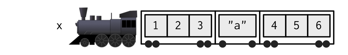
Vectors

All elements must be the same type

Atomic vectors

c(TRUE, FALSE, TRUE)    # logical

[1]  TRUE FALSE  TRUE

c(1L, 5L, 19L)          # integer

[1]  1  5 19

c(3.14, 1, 1.9e2)       # double

[1]   3.14   1.00 190.00

c("cat", "dog", "fish") # character

[1] "cat"  "dog"  "fish"

L suffix for integers hierarchical order of types: logical < integer < double < character

Coercion

Automatic coercion

x <- c(1, "dog")
mode(x)

[1] "character"

x

[1] "1"   "dog"

Deliberate coercion

as.numeric(x)

[1]  1 NA

Predict the outcome of

c(1, FALSE)

[1] 1 0

c("a", 1)

[1] "a" "1"

c(TRUE, 1L)

[1] 1 1

Subsetting a vector

x <- c(5, 1, 4, 7)
x[2]       # extract single element

[1] 1

x[c(1, 3)] # extract multiple elements

[1] 5 4

x[-2]      # remove elements

[1] 5 4 7

x[x > 5]   # logical test

[1] 7

Extract from

x <- c(1, 10, 3, 5, 7)

• first element
• last element
• second and third element
• everything but the second and third element
• element with a value less than 5

Matricies

2 dimensional

All elements same type

m <- matrix(1:9, nrow = 3)
m

     [,1] [,2] [,3]
[1,]    1    4    7
[2,]    2    5    8
[3,]    3    6    9

Arrays can have 3+ dimensions

Arrays are mind-melting

Subsetting a matrix

m

     [,1] [,2] [,3]
[1,]    1    4    7
[2,]    2    5    8
[3,]    3    6    9

[row_indices, column_indices]

m[1:2, 2]

[1] 4 5

Lists

Each element of a list can be a different type

x <- list(
  1:5,
  "b",
  c(TRUE, FALSE)
)

str(x)

List of 3
 $ : int [1:5] 1 2 3 4 5
 $ : chr "b"
 $ : logi [1:2] TRUE FALSE

x

[[1]]
[1] 1 2 3 4 5

[[2]]
[1] "b"

[[3]]
[1]  TRUE FALSE

Lists are very important

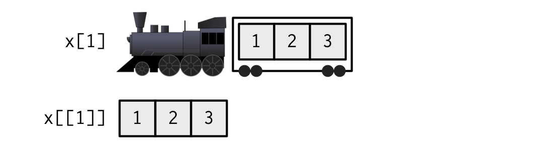
Subsetting a list

x <- list(1:3, "a", 4:6)

Can make a smaller list, or extract contents of a carriage

x

[[1]]
[1] 1 2 3

[[2]]
[1] "a"

[[3]]
[1] 4 5 6

x[1]   # list with one element

[[1]]
[1] 1 2 3

x[1:2] # list with first two elements

[[1]]
[1] 1 2 3

[[2]]
[1] "a"

x[[1]] # content of first element

[1] 1 2 3

Named lists

x <- list(a = 1:3, b = "a", c = 4:6)
x

$a
[1] 1 2 3

$b
[1] "a"

$c
[1] 4 5 6

Extract vector “a”

x$a

[1] 1 2 3

Many functions return named lists eg lm, glm, t-test

Data frames and tibbles

rectangular data structure - 2-dimensions

columns can have different type of object

special type of list where all vectors have same length

Tibbles are better behaved version of data.frame

library(tibble) # part of tidyverse
df2 <- tibble(x = 1:3, y = letters[1:3])
df2

# A tibble: 3 × 2
      x y    
  <int> <chr>
1     1 a    
2     2 b    
3     3 c    

Data.frames have row and column names

names(df2)

[1] "x" "y"

rownames(df2) # not supported by tibbles - use a column instead

[1] "1" "2" "3"

Subsetting a tibble

With square brackets

df2[1, 2]

# A tibble: 1 × 1
  y    
  <chr>
1 a    

With column names

df2$y

[1] "a" "b" "c"

Which method is safer?

Can also use dplyr package.

Control flow

if statements for choice

if (logical_condition) {
  # run this code if logical_condition is true
} else {
  # run this code if logical_condition is false
}

else is optional

use ifelse() or dplyr::case_when() for vectorised if

Boolean logic

logical conditions can be combined

animal <- "cat"
number <- 3

• && AND - TRUE if both TRUE
• || OR - TRUE if either TRUE
• ! NOT - TRUE if FALSE (or use != for not equal)

animal == "cat" && number == 7

[1] FALSE

animal == "cat" || number == 7

[1] TRUE

!animal == "cat" || number == 7

[1] FALSE

!(animal == "cat" || number == 7)

[1] FALSE

Vectorised Boolean logic

&& and || return a single TRUE/FALSE

Useful for if statements

& and | return a vector of TRUE/FALSE

Useful with ifelse() or dplyr::case_when()

a <- 1:10
b <- rep(c("cat", "dog"), 5)

a > 5 && b == "dog" # gives error

Error in a > 5 && b == "dog": 'length = 10' in coercion to 'logical(1)'

a > 5 & b == "dog"

 [1] FALSE FALSE FALSE FALSE FALSE  TRUE FALSE  TRUE FALSE  TRUE

loops

Often don’t need an explicit loop - R is vectorised

a <- c(5, 1, 4, 6)
b <- c(1, 7, 3, 4)
a + b

[1]  6  8  7 10

for loops

for loops iterate over elements of a vector

for (element in vector){
  # run code here
}

for (i in 1:3) {
  i ^ 2
}

for pitfalls

Need to pre-allocate space or slow

n <- 10
result <- numeric(10)
for (i in 1:n) {
  result[i] <- rnorm(1)
}

Rarely need a loop - purrr::map(), apply() generally cleaner

Better iteration with `map()`

library(purrr) # part of tidyverse
lst <- list(a = 1:3, b = c(4, 7), c = 5:9)
map(lst, mean)

$a
[1] 2

$b
[1] 5.5

$c
[1] 7

map_dbl(lst, mean) # returns vector of doubles

  a   b   c 
2.0 5.5 7.0 

apply() for iterating over rows/columns of a matrix

Style

Code is communication

• With your computer

• With your collaborators

“Your closest collaborator is you six months ago but you don’t reply to email.” — Paul Wilson

• With reviewers/examiners

Need understandable code

Goodstylemakescodeeasiertoread

Journal code archiving requirements

Nature Journals

A condition of publication in a Nature Portfolio journal is that authors are required to make materials, data, code, and associated protocols promptly available to readers without undue qualifications.

Canadian Journal of Fisheries and Aquatic Sciences

it is a condition for publication of accepted manuscripts at CJFAS that authors make publicly available all data and code needed to reproduce those results (including code to reproduce statistical results, simulation results, and figures) via an online data repository.

Tidy code

The only way to write good code is to write tons of shitty code first. Feeling shame about bad code stops you from getting to good code

— Hadley Wickham (@hadleywickham) 17 April 2015

• Makes code easier to read
• Makes code easier to debug

Make your own style - but be consistent

Tidyverse style guide

Naming Things

“There are only two hard things in Computer Science: cache invalidation and naming things.”

— Phil Karlton

• Names can contain letters, numbers, “_” and “.”
• Names must begin with a letter or “.”
• Avoid using names of existing functions - confusing
• Make names concise yet meaningful
• Reserved words include TRUE, for, if

Which of these are valid names in R

• min_height
• max.height
• _age
• .mass
• MaxLength
• min-length
• FALSE
• true
• 2widths
• celsius2kelvin
• plot
• T

Names can be too long

“The church of St. Mary of the pool of the white hazels near to the fierce whirlpool and the church of St. Tysilio of the red cave”

Rob Koster - CC BY-SA 3.0

Or too short

k

Common in old FORTRAN code - save memory with short names

exceptions

• counter in a for loop
• main object in a function

Naming convensions

camelCase 🐫	UpperCamelCase	snake_case 🐍
billLengthMM	BillLengthMM	bill_length_mm
bergenWeather2022	BergenWeather2022	bergen_weather_2022
dryMassG	DryMassG	dry_mass_g
makeWeatherPlot	MakeWeatherPlot	make_weather_plot

White-space is free!

Place spaces

• around infix operators (|>, +, -, <-, )
• around = in function calls
• after commas not before

Good

gentoo <- filter(penguins, species == "Gentoo", body_mass_g >= 300)

Bad

gentoo<-filter(penguins,species=="Gentoo",body_mass_g>=300)

Split long commands over multiple lines

penguins |> 
  group_by(species) |> 
  summarise(
    max_mass = max(body_mass_g),
    mean_bill_length = mean(bill_length_mm),
   .groups = "drop"
  )

Aim for a maximum line length of 80 characters

Indentation makes code more readable

Good

positive <- function(x) {
  if (is.null(dim(x))) {
    x[x > 0]
  } else{
    x[, colSums(x) > 0, drop  = FALSE]
  }
}

Bad

positive <- function(x){
if(is.null(dim(x)))
{x[x >0]} 
else{
x[, colSums(x) > 0, drop  = FALSE]
}}

Stylers & lintr

Use styler package to edit code to meet style guide.

Use lintr package for static code analysis, including style check

Demo

Comments

Use # to start comments.

Help you and others to understand what you did

Comments should explain the why, not the what.

# Bad
# remove line 37 of the penguins dataset
penguins <- penguins[-37, ]

Try to make code self-documenting with descriptive object names

Comments for navigation

Helps you find your way around a script

#### Load data ####
...

#### Plot data ####
...

No magic numbers

# Bad
x <- c(1, 5, 6, 3, 6)
mean(x)

[1] 4.2

x[x > 4.2]

[1] 5 6 6

# Good
x <- c(1, 5, 6, 3, 6)
x_mean <- mean(x)
x[x > x_mean]

[1] 5 6 6

Split analyses over multiple files

Long scripts become difficult to navigate

Fix by moving parts of the code into different files

For example:

• data import code to “loadData.R”
• functions to “functions.R”

Import with

source("loadData.R")
source("functions.R")

Don’t repeat yourself

Repeated code is hard to maintain

Make repeated code into functions.

my_fun <- function(arg1) {arg1 ^ 2}
my_fun(7)

Single place to maintain

Encapsulate code

make_figure_one <- function() {
  ggplot(penguins, aes(x = bill_length_mm)) +
    geom_histogram()
}

make_figure_one()