Data manipulation

Bio300B Lecture 3

Richard J. Telford (Richard.Telford@uib.no)

Institutt for biovitenskap, UiB

25 September 2024

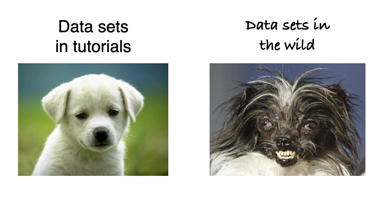
Data cleaning

• Critical
• Time consuming
• Do in code for reproducibility
• Often not taught

Figure from towards_AI

Penguins

library(palmerpenguins)
penguins

# A tibble: 344 × 8
  species island    bill_length_mm bill_depth_mm flipper_length_mm body_mass_g
  <fct>   <fct>              <dbl>         <dbl>             <int>       <int>
1 Adelie  Torgersen           39.1          18.7               181        3750
2 Adelie  Torgersen           39.5          17.4               186        3800
# ℹ 342 more rows
# ℹ 2 more variables: sex <fct>, year <int>

palmerpenguins: Palmer Archipelago (Antarctica) Penguin Data

Size measurements for adult foraging Adélie, Chinstrap, and Gentoo penguins observed on islands in the Palmer Archipelago, Antarctica.

Importing data

First step of almost any data analysis

• read_delim() from readr package
• read_excel() from readxl package

Lots of arguments to help import data correctly

Find the data rectangle and import just that.

Paths

Use RStudio projects

Use relative paths

# absolute path - bad
"c://users/richard/documents/biostats/data/data.csv"
# relative path - good
"data/data.csv"

Pipes

Analysis:

• With penguins data
• Drop rows with NA sex
• find mean bill length per species per sex

First solution

Nested functions

summarise(
  group_by(drop_na(penguins, sex), species, sex), 
  bill_length_mean = mean(bill_length_mm),
  .groups = "drop")

# A tibble: 6 × 3
  species sex    bill_length_mean
  <fct>   <fct>             <dbl>
1 Adelie  female             37.3
2 Adelie  male               40.4
# ℹ 4 more rows

Second solution

p <- drop_na(penguins, sex)
p <- group_by(p, species, sex)
p <- summarise(p,
         bill_length_mean = mean(bill_length_mm),
        .groups = "drop")

Third solution

p_1 <- drop_na(penguins, sex)
p_2 <- group_by(p_1, species, sex)
p_3 <- summarise(p_2,
         bill_length_mean = mean(bill_length_mm),
        .groups = "drop")

pipe solution

p <- penguins |> 
  drop_na(sex) |> 
  group_by(species, sex) |> 
  summarise(
    bill_length_mean = mean(bill_length_mm),
    .groups = "drop")

Pipe puts result of left hand side into first available argument on right hand side

• |> native R pipe
• %>% magrittr pipe

Tidy data

“Happy families are all alike; every unhappy family is unhappy in its own way”
— Tolstoy

Tidy data

• easy to work with
• use standard tools to manipulate, visualise and analyse
• can reuse code from other projects

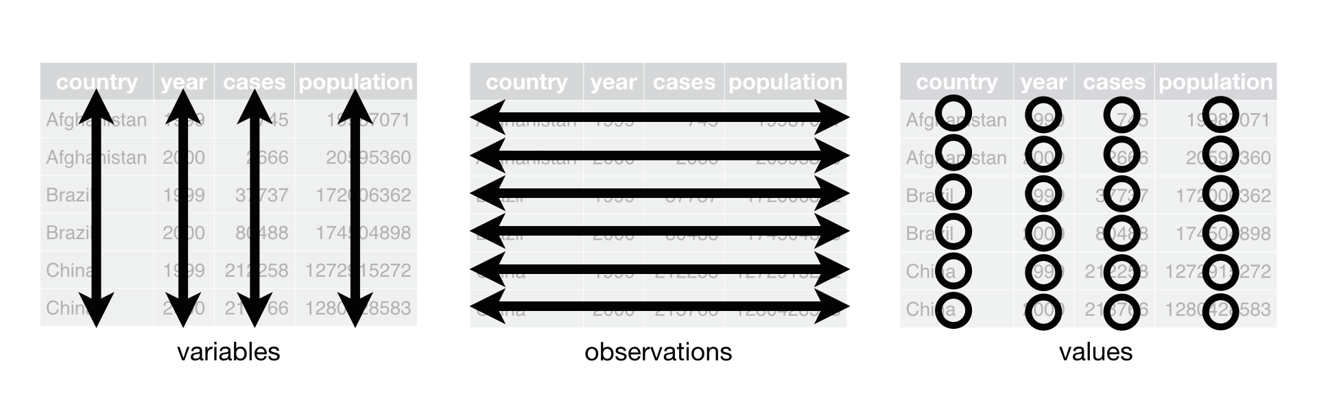
What are tidy data

• Every column is a variable.
• Every row is an observation.
• Every cell is a single value.

Wickham (2014) Tidy data

Untidy data

Date	17.06.2016	21.06.2016	23.06.2016	26.06.2016
Time	10:00	11:00	11:00	13:00
Weather	Sunny_PartlyCloudy	Cloudy_Fog	Cloudy_Sunny	Cloudy_Rainy_Windy_Fog
Observer	LV_AH	LV	LV	LV
E01a	0	NA	0	0
E01b	0	NA	0	0
E01c	0	NA	0	0
E01d	0	NA	0	0
E01e	0	NA	0	0

The heart of your analysis pipeline

Reshaping data

Long data vs wide data

Wide data

mites # part of vegan::mite

  sample Brachy PHTH HPAV RARD
1      1     17    5    5    3
2      2      2    7   16    0
3      3      4    3    1    1
4      4     23    7   10    2
5      5      5    8   13    9

Wide format data needed for ordinations and related methods used in Bio303

Making longer data

tidyr::pivot_longer()

mites_long <- mites |> 
  pivot_longer(cols = Brachy:RARD, 
               names_to = "taxon", 
               values_to = "count")
mites_long

# A tibble: 20 × 3
   sample taxon  count
    <int> <chr>  <int>
 1      1 Brachy    17
 2      1 PHTH       5
 3      1 HPAV       5
 4      1 RARD       3
 5      2 Brachy     2
 6      2 PHTH       7
 7      2 HPAV      16
 8      2 RARD       0
 9      3 Brachy     4
10      3 PHTH       3
# ℹ 10 more rows

Making wider data

tidyr::pivot_wider()

mites_wide <- mites_long |> 
  pivot_wider(names_from = "taxon", 
              values_from = "count")
mites_wide

# A tibble: 5 × 5
  sample Brachy  PHTH  HPAV  RARD
   <int>  <int> <int> <int> <int>
1      1     17     5     5     3
2      2      2     7    16     0
3      3      4     3     1     1
4      4     23     7    10     2
5      5      5     8    13     9

Processing data with dplyr

Key dplyr functions

• select()
• filter()
• mutate()
• summarise()
• group_by()

Normally load dplyr with library(tidyverse)

Selecting columns

dplyr::select()

penguins |> 
  select(species, bill_length_mm)

# A tibble: 344 × 2
  species bill_length_mm
  <fct>            <dbl>
1 Adelie            39.1
2 Adelie            39.5
# ℹ 342 more rows

penguins |> 
  select(-bill_length_mm, -bill_depth_mm)

# A tibble: 344 × 6
  species island    flipper_length_mm body_mass_g sex     year
  <fct>   <fct>                 <int>       <int> <fct>  <int>
1 Adelie  Torgersen               181        3750 male    2007
2 Adelie  Torgersen               186        3800 female  2007
# ℹ 342 more rows

Selecting adjacent columns

penguins |> 
  select(bill_length_mm:body_mass_g)

# A tibble: 344 × 4
  bill_length_mm bill_depth_mm flipper_length_mm body_mass_g
           <dbl>         <dbl>             <int>       <int>
1           39.1          18.7               181        3750
2           39.5          17.4               186        3800
# ℹ 342 more rows

penguins |> 
  select(-(bill_length_mm:body_mass_g))

# A tibble: 344 × 4
  species island    sex     year
  <fct>   <fct>     <fct>  <int>
1 Adelie  Torgersen male    2007
2 Adelie  Torgersen female  2007
# ℹ 342 more rows

Select helpers

ends_with()

penguins |> 
  select(species, ends_with("mm"))

# A tibble: 344 × 4
  species bill_length_mm bill_depth_mm flipper_length_mm
  <fct>            <dbl>         <dbl>             <int>
1 Adelie            39.1          18.7               181
2 Adelie            39.5          17.4               186
# ℹ 342 more rows

• starts_with()
• contains()
• matches() regular expressions

Your turn

names(penguins)

[1] "species"           "island"            "bill_length_mm"   
[4] "bill_depth_mm"     "flipper_length_mm" "body_mass_g"      
[7] "sex"               "year"             

How would you make a data frame with

• just species and island
• without year
• with species and the length measurements

Filtering rows

dplyr::filter()

penguins |> filter(species == "Gentoo")

# A tibble: 124 × 8
  species island bill_length_mm bill_depth_mm flipper_length_mm body_mass_g
  <fct>   <fct>           <dbl>         <dbl>             <int>       <int>
1 Gentoo  Biscoe           46.1          13.2               211        4500
2 Gentoo  Biscoe           50            16.3               230        5700
# ℹ 122 more rows
# ℹ 2 more variables: sex <fct>, year <int>

One or more logical statements

• ==
• >=
• <
• !=

separate statements with commas

near()

Problem:

sqrt(2) ^ 2 == 2

[1] FALSE

sqrt(2) ^ 2 - 2

[1] 4.440892e-16

\(\sqrt{2}\) is irrational - cannot be perfectly represented

Solution:

near(sqrt(2) ^ 2, 2)

[1] TRUE

data stored as doubles - finite precision

%in%

Problem

penguins |> 
  filter(species == "Gentoo" | species == "Chinstrap")

# A tibble: 192 × 8
  species island bill_length_mm bill_depth_mm flipper_length_mm body_mass_g
  <fct>   <fct>           <dbl>         <dbl>             <int>       <int>
1 Gentoo  Biscoe           46.1          13.2               211        4500
2 Gentoo  Biscoe           50            16.3               230        5700
# ℹ 190 more rows
# ℹ 2 more variables: sex <fct>, year <int>

• | OR

Solution

penguins |> 
  filter(species %in% c("Gentoo", "Chinstrap"))

# A tibble: 192 × 8
  species island bill_length_mm bill_depth_mm flipper_length_mm body_mass_g
  <fct>   <fct>           <dbl>         <dbl>             <int>       <int>
1 Gentoo  Biscoe           46.1          13.2               211        4500
2 Gentoo  Biscoe           50            16.3               230        5700
# ℹ 190 more rows
# ℹ 2 more variables: sex <fct>, year <int>

between()

Problem

penguins |> 
  filter(body_mass_g >= 2000, body_mass_g <= 3000)

# A tibble: 11 × 8
  species island bill_length_mm bill_depth_mm flipper_length_mm body_mass_g
  <fct>   <fct>           <dbl>         <dbl>             <int>       <int>
1 Adelie  Dream            37            16.9               185        3000
2 Adelie  Dream            37.5          18.9               179        2975
# ℹ 9 more rows
# ℹ 2 more variables: sex <fct>, year <int>

Solution

penguins |> 
  filter(between(body_mass_g, left = 2000, right = 3000))

# A tibble: 11 × 8
  species island bill_length_mm bill_depth_mm flipper_length_mm body_mass_g
  <fct>   <fct>           <dbl>         <dbl>             <int>       <int>
1 Adelie  Dream            37            16.9               185        3000
2 Adelie  Dream            37.5          18.9               179        2975
# ℹ 9 more rows
# ℹ 2 more variables: sex <fct>, year <int>

Partial string matches

Problem

Want to filter by partial text match

solution: stringr package

penguins |> 
  filter(str_detect(species, "G"))

# A tibble: 124 × 8
  species island bill_length_mm bill_depth_mm flipper_length_mm body_mass_g
  <fct>   <fct>           <dbl>         <dbl>             <int>       <int>
1 Gentoo  Biscoe           46.1          13.2               211        4500
2 Gentoo  Biscoe           50            16.3               230        5700
# ℹ 122 more rows
# ℹ 2 more variables: sex <fct>, year <int>

Regular expressions for more powerful matching.

How would you

penguins

# A tibble: 344 × 8
  species island    bill_length_mm bill_depth_mm flipper_length_mm body_mass_g
  <fct>   <fct>              <dbl>         <dbl>             <int>       <int>
1 Adelie  Torgersen           39.1          18.7               181        3750
2 Adelie  Torgersen           39.5          17.4               186        3800
# ℹ 342 more rows
# ℹ 2 more variables: sex <fct>, year <int>

Get a data frame with

• Male Gentoo penguins
• Penguins with a mass > 1000 g
• Penguins from Dream or Biscoe Island

Mutating columns with mutate()

Make a new column or change an existing column

penguins |> mutate(
  species = tolower(species),
  body_mass_kg = body_mass_g/1000,
  bill_ratio = bill_length_mm/bill_depth_mm
  )

# A tibble: 344 × 10
  species island    bill_length_mm bill_depth_mm flipper_length_mm body_mass_g
  <chr>   <fct>              <dbl>         <dbl>             <int>       <int>
1 adelie  Torgersen           39.1          18.7               181        3750
2 adelie  Torgersen           39.5          17.4               186        3800
# ℹ 342 more rows
# ℹ 4 more variables: sex <fct>, year <int>, body_mass_kg <dbl>,
#   bill_ratio <dbl>

Useful functions for mutate

• mutate character columns with stringr, glue
• mutate factor columns with forcats
• mutate dates with lubridate

Summarising data with summarise

penguins |> 
  summarise(
    max_mass = max(body_mass_g, na.rm = TRUE),
    mean_bill_length = mean(bill_length_mm, na.rm = TRUE)
  )

# A tibble: 1 × 2
  max_mass mean_bill_length
     <int>            <dbl>
1     6300             43.9

Useful functions

• limits min() max()
• centre mean() median()
• spread sd()
• number n() n_distinct()

Grouping data

penguins |> 
  group_by(species, island)

# A tibble: 344 × 8
# Groups:   species, island [5]
  species island    bill_length_mm bill_depth_mm flipper_length_mm body_mass_g
  <fct>   <fct>              <dbl>         <dbl>             <int>       <int>
1 Adelie  Torgersen           39.1          18.7               181        3750
2 Adelie  Torgersen           39.5          17.4               186        3800
# ℹ 342 more rows
# ℹ 2 more variables: sex <fct>, year <int>

Mutate and summarise now work per group

Mutating grouped data

Analysis per group

penguins |> 
  group_by(species) |> 
  mutate(bill_length_mean = mean(bill_length_mm, na.rm = TRUE),
         bill_length_centred = bill_length_mm - bill_length_mean)

# A tibble: 344 × 10
# Groups:   species [3]
  species island    bill_length_mm bill_depth_mm flipper_length_mm body_mass_g
  <fct>   <fct>              <dbl>         <dbl>             <int>       <int>
1 Adelie  Torgersen           39.1          18.7               181        3750
2 Adelie  Torgersen           39.5          17.4               186        3800
# ℹ 342 more rows
# ℹ 4 more variables: sex <fct>, year <int>, bill_length_mean <dbl>,
#   bill_length_centred <dbl>

Summarising grouped data

Summary per group

penguins |> 
  group_by(species) |> 
  summarise(
    max_mass = max(body_mass_g),
    mean_bill_length = mean(bill_length_mm),
   .groups = "drop"
  )

# A tibble: 3 × 3
  species   max_mass mean_bill_length
  <fct>        <int>            <dbl>
1 Adelie          NA             NA  
2 Chinstrap     4800             48.8
3 Gentoo          NA             NA  

NA - Not available - missing data

NA are contagious: what is 5 + NA?

penguins |> 
  group_by(species) |> 
  summarise(
    max_mass = max(body_mass_g, na.rm = TRUE),
    mean_bill_length = mean(bill_length_mm, na.rm = TRUE),
   .groups = "drop"
  )

# A tibble: 3 × 3
  species   max_mass mean_bill_length
  <fct>        <int>            <dbl>
1 Adelie        4775             38.8
2 Chinstrap     4800             48.8
3 Gentoo        6300             47.5

Counting rows

penguins |> 
  count(species, island, sex)

# A tibble: 13 × 4
  species island sex        n
  <fct>   <fct>  <fct>  <int>
1 Adelie  Biscoe female    22
2 Adelie  Biscoe male      22
# ℹ 11 more rows

penguins |> 
  group_by(species, island, sex) |> 
  summarise(n = n(), .groups = "drop")

# A tibble: 13 × 4
  species island sex        n
  <fct>   <fct>  <fct>  <int>
1 Adelie  Biscoe female    22
2 Adelie  Biscoe male      22
# ℹ 11 more rows

Mutating joins

Merge two tibbles

left_join()

band_members

# A tibble: 3 × 2
  name  band   
  <chr> <chr>  
1 Mick  Stones 
2 John  Beatles
3 Paul  Beatles

band_instruments

# A tibble: 3 × 2
  name  plays 
  <chr> <chr> 
1 John  guitar
2 Paul  bass  
3 Keith guitar

. . .

band_members %>% 
  left_join(band_instruments, by = join_by(name))

# A tibble: 3 × 3
  name  band    plays 
  <chr> <chr>   <chr> 
1 Mick  Stones  <NA>  
2 John  Beatles guitar
3 Paul  Beatles bass  

Other joins

• inner_join()
• full_join()

Filtering joins

#semi join
band_members %>% 
  semi_join(band_instruments, by = join_by(name))

# A tibble: 2 × 2
  name  band   
  <chr> <chr>  
1 John  Beatles
2 Paul  Beatles

#anti join
band_members %>% 
  anti_join(band_instruments, by = join_by(name))

# A tibble: 1 × 2
  name  band  
  <chr> <chr> 
1 Mick  Stones

Further reading

Wickham et al. (2023) R for Data Science

Wickham, H. Advanced R