[1] 0.5951Linear Regression 1
Bio300B Lecture 7
Richard J. Telford (Richard.Telford@uib.no)
Institutt for biovitenskap, UiB
29 September 2025
Bivariate descriptive statistics
Measures of association
- covariance
- correlation
Use with
- two continuous variables
- paired data
- unclear direction of causality
Covariance
Association between two variables
\(S_{xy} = \frac{\Sigma (x_i - \mu_x)(y_i - \mu_y)}{n - 1}\)
\(S_{xy} = S_{yx}\)
- -inf, 0, +inf
- + = positive association
- - = negative association
cov()
Correlation
Pearson coefficient of correlation
Standardised association
- \(S_{xy}\) - covariance of x & y
- \(S_x^2\) - variance of x
- \(S_y^2\) - variance of y
\(r_{xy} = \frac{S_{xy}}{\sqrt{S_x^2S_y^2}}\)
\(r_{xy} = r_{yx}\)
- -1, 0, +1
- + = positive association
- - = negative association
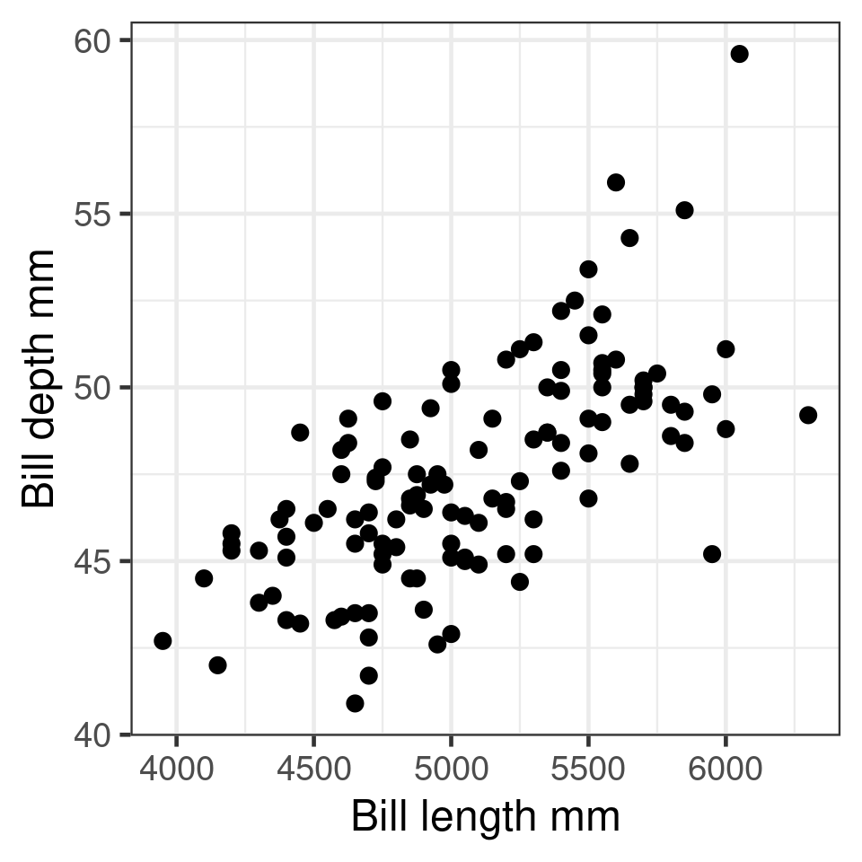
Correlations in R
Correlation between two variables
Correlation matrix
                  bill_length_mm bill_depth_mm flipper_length_mm body_mass_g
bill_length_mm            1.0000       -0.2351            0.6562      0.5951
bill_depth_mm            -0.2351        1.0000           -0.5839     -0.4719
flipper_length_mm         0.6562       -0.5839            1.0000      0.8712
body_mass_g               0.5951       -0.4719            0.8712      1.0000
\(R^2\)
Coefficient of determination
\[R^2 = r^2\]
- 0 – 1
- proportion of variance explained
- \(R^2\) = 0.5, 50% of variation in data explained
Testing a Correlation
    Pearson's product-moment correlation

data:  penguins$bill_length_mm and penguins$body_mass_g
t = 14, df = 340, p-value <2e-16
alternative hypothesis: true correlation is not equal to 0
95 percent confidence interval:
 0.5220 0.6595
sample estimates:
   cor
0.5951
Not robust to outliers
- Non-parametric correlation (Spearman Rank, Kendall Tau)
- Bootstrap estimation of confidence interval
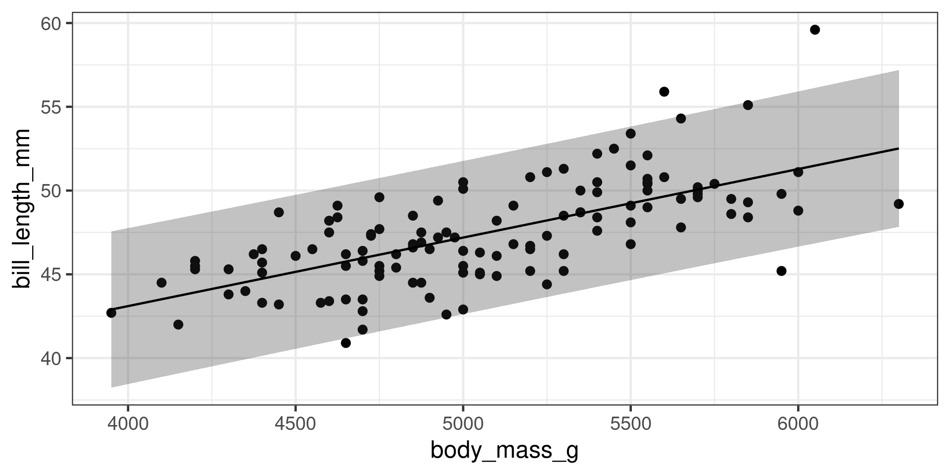
Least squares regression
Describe relationship between response y and predictor x \[y = β_0 + β_1x\]
We want the parameters \(\beta\)
\[y_i = \beta_0 + \beta_1x_i + \varepsilon_i \]
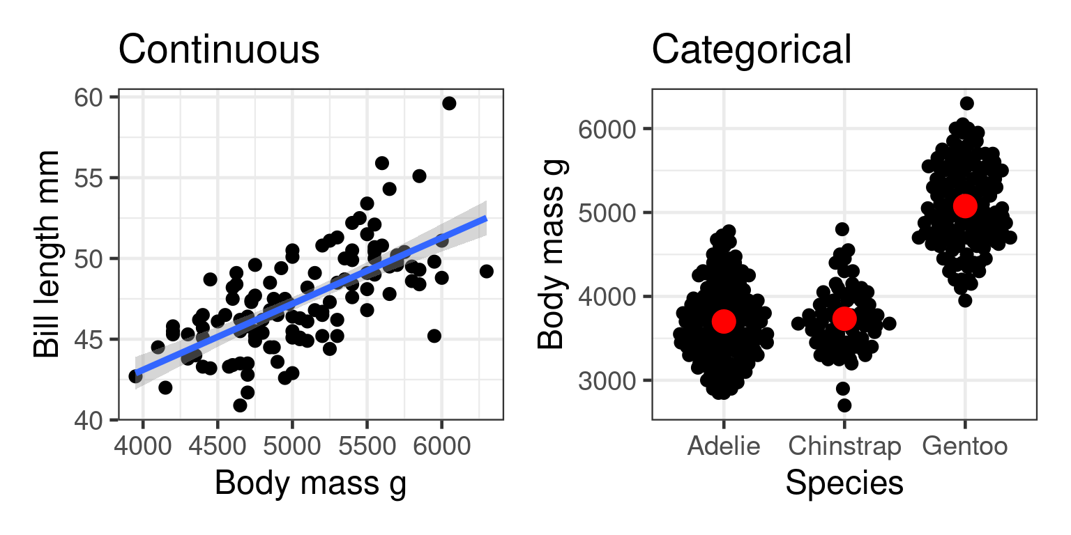
- \(y\) = continuous response
- \(x\) = continuous or categorical predictor
- \(i = 1, ..., n\) observations - \((xi, yi)\) observation pairs
- \(ε_i\) = residual at \(i\)
- \(β_0\) = mean, intercept
- \(β_1\) = effect, slope
Residuals are actual - predicted
Criteria
- \(\varepsilon \sim N(0, \sigma)\)
- \(y \sim N(\mu, \sigma)\)
Use when
Response variable is continuous
Predictor variable(s) are continuous or categorical
Observations are independent
Other assumptions are met
Direction of causality is clear
Want to make predictions
Want effect size as slope or differences between groups
Correlation or linear model?
Studying foraminifera test composition and temperature
- Experiment with forams in tanks at different temperatures.
- foram Mg concentration, tank temperature
- foram Mg concentration, foram Ba concentration
- Observational study of forams collected from the ocean.
- foram Mg concentration, Ocean temperature
- Ocean temperature, ocean Mg concentration
- foram Mg concentration, foram species
Which distribution matters?
#| '!! shinylive warning !!': |
#|   shinylive does not work in self-contained HTML documents.
#|   Please set `embed-resources: false` in your metadata.
#| label: ydistribution-lm-app
#| standalone: true
#| viewerHeight: 600

library(shiny)

ui <-  fluidPage(
  # Application title
  titlePanel("Which distribution is important?"),
  sidebarLayout(
    sidebarPanel(
      radioButtons("dist", "Predictor distributor", choices = c("Normal", "Skewed", "Bimodal"), selected = "Normal"),
      checkboxInput("show_residuals", label = "Show residuals", value = FALSE),
      radioButtons("residual_plot", "Residual plot", choices = c("None", "Histogram", "QQplot"), selected = "None")
    ),
    # Show a plot of the generated distribution
    mainPanel(
      plotOutput("distPlot")
    )
  ))

  horizHist <- function(
    Data,
    breaks="Sturges",
    freq=TRUE,
    plot=TRUE,
    col=par("bg"),
    border=par("fg"),
    las=1,
    xlab=if(freq)"Frequency" else "Density",
    main=paste("Histogram of",deparse(substitute(Data))),
    ylim=range(HBreaks),
    labelat=pretty(ylim),
    labels=labelat,
    ... )
  {
    a <- hist(Data, plot=FALSE, breaks=breaks)
    HBreaks <- a$breaks
    hpos <- function(Pos) (Pos-HBreaks[1])*(length(HBreaks)-1)/ diff(range(HBreaks))
    if(plot)
    {
      barplot(if(freq)a$counts else a$density, space=0, horiz=TRUE, ylim=hpos(ylim), col=col, border=border,
              xlab=xlab, main=main, ...)
    }
  } # End of function

server <- function(input, output, session) {
  x <- reactive(switch(input$dist,
                Normal = rnorm(50),
                Skewed = exp(rnorm(50)),
                Bimodal = c(rnorm(25, mean = 1, sd = 0.4), rnorm(25, mean = 5, sd = 0.4))
        ))
  y <- reactive(rnorm(length(x()), mean = x()))
  mod <- reactive(lm(y() ~ x()))

  output$distPlot <- renderPlot({


    layout(mat = matrix(c(1, 2, 4, 0, 3, 0),
                        nrow = 3,
                        ncol = 2),
           heights = c(1, 3, 3),    # Heights of the two rows
           widths = c(3, 1))     # Widths of the two columns
    par(mar=c(1.2,2,2,1),  cex = 1.3, tcl = -0.1, mgp = c(1.5, 0.2, 0))
    par(mar = c(0, 3, 0, 0))
    hist(x(), axes = FALSE, main = "", ylab = "", xlab = "", breaks = 10)
    par(mar = c(3, 3, 0, 0))
    plot(x(), y(), xlab = "Predictor", ylab = "Response")
    abline(coef = coef(mod()))
    if (input$show_residuals) {
      segments(x0 = x(), y0 = y(), x1 = x(), y1 = fitted(mod()))
    }
    par(mar = c(3, 0.2, 0, 0))
    horizHist(y(), axes = FALSE, main = "", ylab = "", xlab = "", col = "lightgrey", breaks = 10)

    if (input$residual_plot == "Histogram") {
        par(mar = c(3, 3, 1, 0))
        hist(resid(mod()), freq = FALSE)
        x_norm <- seq(-10, 10, length.out = 100)
        lines(x_norm, dnorm(x_norm, mean = 0, sd = sd(resid(mod()))), col = "#832424", xlab = "Residuals", main = "Histogram of residuals")
    } else if (input$residual_plot == "QQplot") {
        par(mar = c(3, 3, 1, 0))
        plot(mod(), which = 2, id.n = 0)
    }

  })
}

shinyApp(ui, server)
Estimating \(\beta\)
Choose \(\beta\) that minimise the sum of squares of residuals
\[\sum_{i = 1}^{n}\varepsilon_i^2 = \sum_{i = 1}^{n}(y_i - (\beta_0 + \beta_1x_i))^2\]
#| '!! shinylive warning !!': |
#|   shinylive does not work in self-contained HTML documents.
#|   Please set `embed-resources: false` in your metadata.
#| label: regression-line-ss-app
#| standalone: true
#| viewerHeight: 600
library(shiny)

ui <-  fluidPage(
        # Application title
      titlePanel("Minimise the sum of squared residuals"),
      sidebarLayout(
          sidebarPanel(
            radioButtons("residuals", "Show residuals", choices = c("None", "Residuals", "Squared-residuals"), selected = "None"),
            checkboxInput("best", "Show best model"),
            textOutput("slope"),
            textOutput("intercept")
         ),
            # Show a plot of the generated distribution
          mainPanel(
             plotOutput("plot", click = "plot_click"),
             h3(textOutput("SumSq"))
          )
))

server <- function(input, output, session) {
  # make some data
  set.seed(Sys.Date())
  data <- data.frame(x = 1:10, y = rnorm(10, 1:10))
  xlab <- "Predictor"
  ylab <- "Response"

  v <- reactiveValues(
    click1 = NULL,  # Represents the first mouse click, if any
    intercept = NULL,    # After two clicks, this stores the intercept
    slope = NULL, # after two clicks, this stores the slope,
    pred = NULL,
    resid = NULL
  )

  # Handle clicks on the plot
 observeEvent(input$plot_click, {
    if (is.null(v$click1)) {
      # We don't have a first click, so this is the first click
      v$click1 <- input$plot_click
    } else {
      # We already had a first click, so this is the second click.
      # Make slope and intercept from the previous click and this one.
      v$slope <- (input$plot_click$y - v$click1$y)/(input$plot_click$x - v$click1$x)
      v$intercept <- (input$plot_click$y + v$click1$y)/2 - v$slope * (input$plot_click$x + v$click1$x)/2

      # predictions & residuals
       v$pred <- v$intercept +  v$slope * data$x
       v$resid <- v$pred - data$y
      # And clear the first click so the next click starts a new line.
      v$click1 <- NULL
    }
  })


 output$plot <- renderPlot({
   par(cex = 1.5, mar = c(3, 3, 1, 1), tcl = -0.1, mgp = c(2, 0.2, 0))
   plot(data, pch = 16, xlab = xlab, ylab = ylab)
   if (input$best) {
     mod <- lm(y ~ x, data = data)
     abline(mod, colour = "navy", lty = "dashed")
   }
   if (!is.null(v$intercept)) {
     abline(a = v$intercept, b = v$slope)
     if (input$residuals == "Residuals") {
       segments(
         x0 = data$x,
         x1 = data$x,
         y0 = data$y,
         y1 = v$pred
       )
     } else if (input$residuals == "Squared-residuals") {
       w   <- par("pin")[1] / diff(par("usr")[1:2])
       h   <- par("pin")[2] / diff(par("usr")[3:4])
       asp <- w/h
       rect(xleft = ifelse(v$resid < 0,  data$x, data$x + v$resid / asp),
            ybottom = ifelse(v$resid < 0, v$pred, data$y),
            xright = ifelse(v$resid < 0, data$x + v$resid / asp, data$x),
            ytop = ifelse(v$resid < 0, data$y, v$pred),
            col = "#83242455", border = "#832424")
     }

   }
 })
 output$SumSq <- renderText({
   if (is.null(v$click1) && is.null(v$intercept)) { # initial state
     "Click on the plot to start a line"
   } else if (!is.null(v$click1)) { #after one click
      "Click again to finsh a line"
   } else if(input$residuals == "None") {
     "Use radio buttons to display residuals"
   } else {
      paste0("Sum of squares = ", signif(sum(v$resid ^ 2), 3))
   }

 })
    output$slope <- renderText({
     if (!is.null(v$slope)) {
       paste0("Slope = ", signif(v$slope, 3))
     } else {
       ""
     }
   })
  output$intercept <- renderText({
     if (!is.null(v$intercept)) {
       paste0("Intercept = ", signif(v$intercept, 3))
     } else {
       ""
     }
   })
}

shinyApp(ui, server)
Calculating \(\beta\)
\[\beta_1 = \frac{s_{xy}}{s_x^2}\] Covariance of xy / variance of x
\[\beta_0 = mean(y) - \beta_1 mean(x)\]
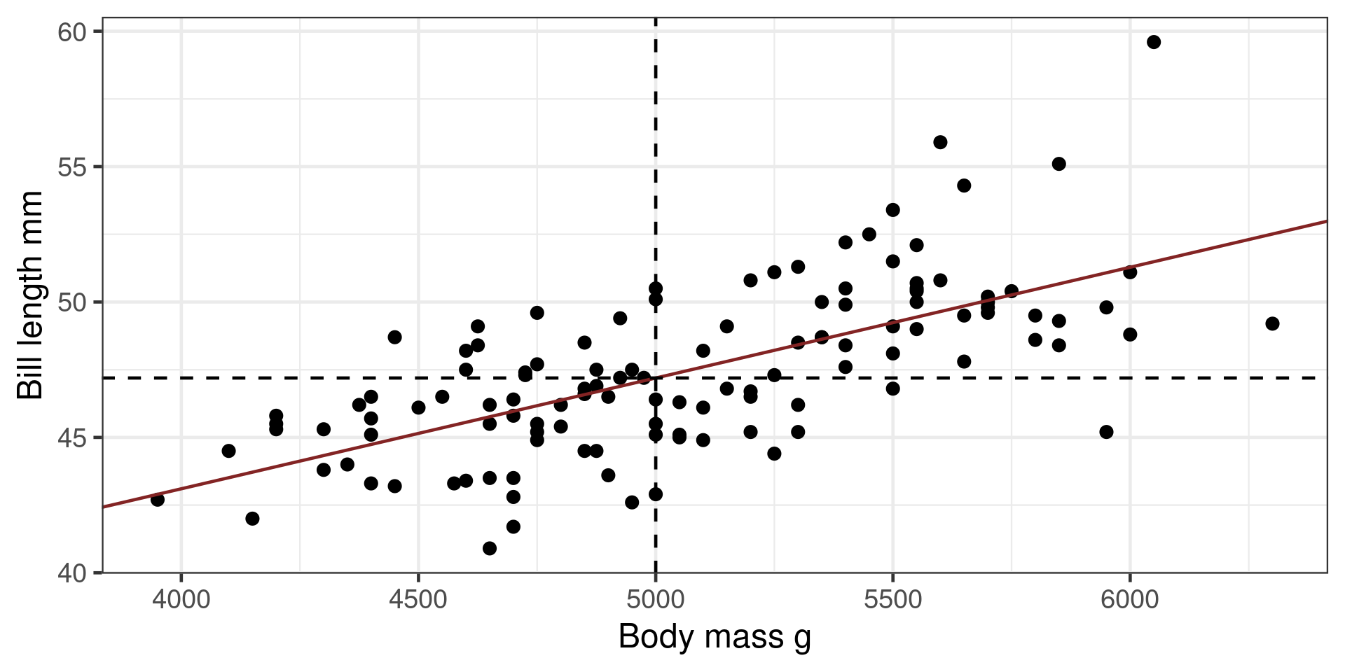
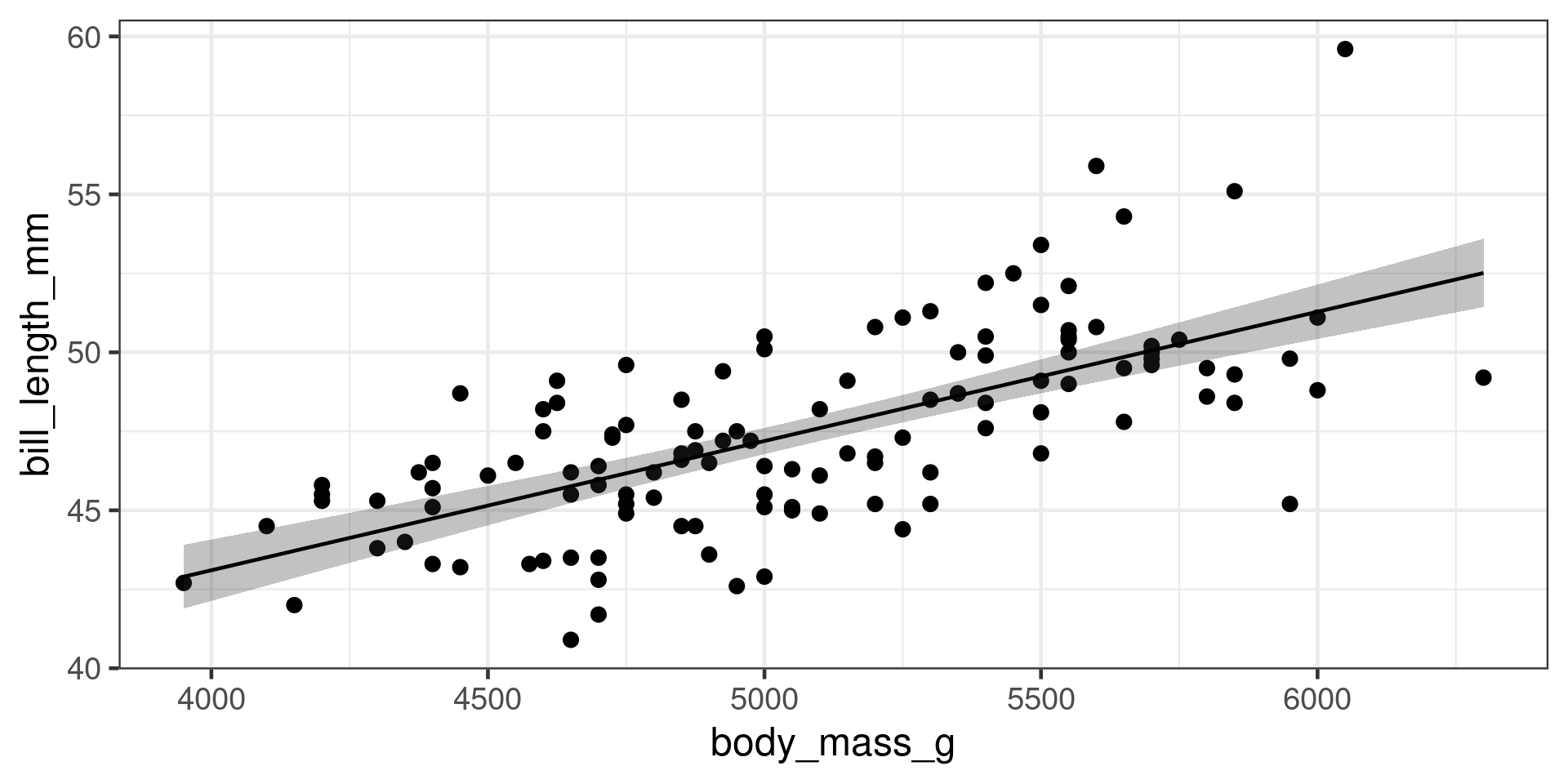
Fitting a least-squares model in R
Summary()
Call:
lm(formula = bill_length_mm ~ body_mass_g, data = gentoo)
Residuals:
Min 1Q Median 3Q Max
-5.880 -1.508 -0.058 1.312 8.111
Coefficients:
Estimate Std. Error t value Pr(>|t|)
(Intercept) 2.67e+01 2.11e+00 12.69 <2e-16 ***
body_mass_g 4.09e-03 4.13e-04 9.91 <2e-16 ***
---
Signif. codes: 0 '***' 0.001 '**' 0.01 '*' 0.05 '.' 0.1 ' ' 1
Residual standard error: 2.3 on 121 degrees of freedom
(1 observation deleted due to missingness)
Multiple R-squared: 0.448, Adjusted R-squared: 0.443
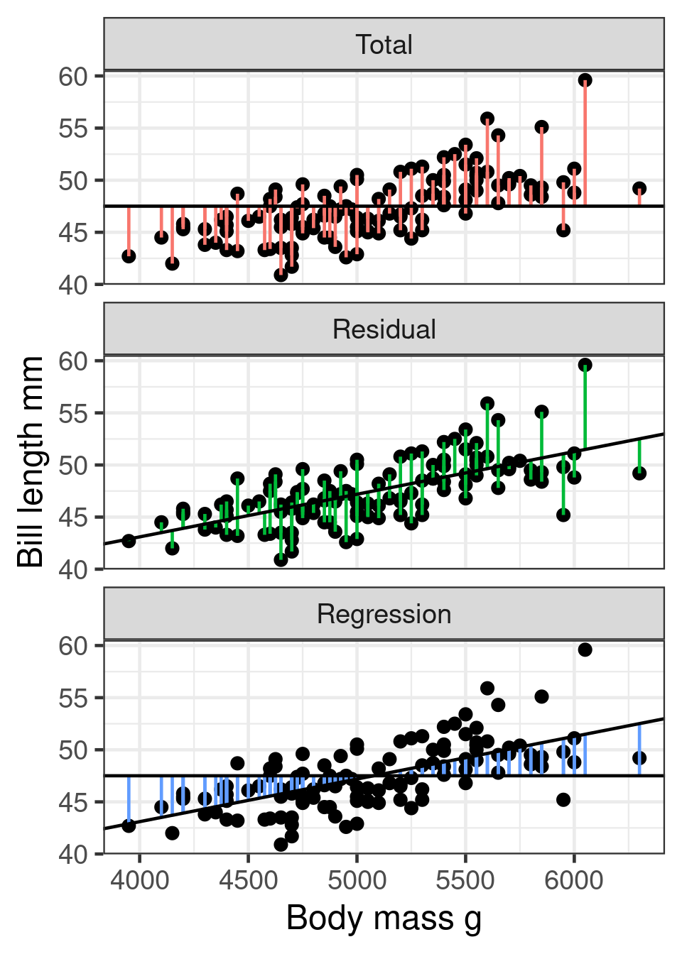
F-statistic: 98.1 on 1 and 121 DF, p-value: <2e-16Variance partitioning
Total sum of squares \(SS_{total}\)
Squared differences of observation from mean
Residual sum of squares \(SS_{residual}\)
Squared differences of observation from regression line
Regression sum of squares \(SS_{regression}\)
Squared differences of regression line from mean
\(R^2\)
Coefficient of determination
Coefficient of multiple correlation
\[R^2 = 1 - \frac{\color{green}{SS_{residual}}}{\color{red}{SS_{total}}}\]
- 0 - 1
- \(R^2\) = 0.5 – 50% of variation in data explained
- Always increases with more predictors
Adjusted \(R^2\)
Corrects for number of parameters
\[
R^2_{adj} = 1 - \frac{(1-R^2)(n-1)}{n-p-1}
\] \(R^2\) = R squared
\(n\) = number of observations
\(p\) = number of parameters
Only increases if useful predictors added
Can be negative
Using Anova
\[F = \frac{\color{blue}{SS_{regression}}/df_{regression}}{\color{green}{SS_{residual}}/df_{residual}}\]
The F distribution
#| '!! shinylive warning !!': |
#|   shinylive does not work in self-contained HTML documents.
#|   Please set `embed-resources: false` in your metadata.
#| label: f-test-app
#| standalone: true
#| viewerHeight: 600

f_dist_app <- function() {
  ui <- page_sidebar(
    # Application title
    title = h1("F distribution"),

    # Sidebar with a slider input for number of bins
    sidebar = sidebar(
      sliderInput(
        "numerator",
        "Regression degrees of freedom:",
        min = 1,
        max = 10,
        round = TRUE,
        value = 1
      ),
      sliderInput(
        "denominator",
        "Residual degrees of freedom:",
        min = 1,
        max = 10,
        round = TRUE,
        value = 5
      ),
      radioButtons(
        "alpha",
        "\u03b1:",
        c("p = 0.05" = "0.05", "p = 0.01" = "0.01")
      )
    ),
    withMathJax(h3(
      "$$F = \\frac{SS_{regression} / df_{regression}}{SS_{residual} / df_{residual}}$$"
    )),
    # Show a plot of the generated distribution
    card(
      plotOutput("distPlot")
    )
  )

  # Define server logic required to draw a histogram
  f_test_server <- function(input, output) {
    output$distPlot <- renderPlot({
      # generate bins based on input$bins from ui.R
      axis_max <- 500
      xmax <- min(
        axis_max,
        qf(
          p = 0.995,
          df1 = input$numerator,
          df2 = input$denominator
        )
      )
      x <- seq(0, ceiling(xmax), length.out = 200)
      y <- df(x, df1 = input$numerator, df2 = input$denominator)
      x <- x[is.finite(y)]
      y <- y[is.finite(y)]

      xthresh <- qf(
        p = 1 - as.numeric(input$alpha),
        df1 = input$numerator,
        df2 = input$denominator
      )
      if (xthresh > axis_max) {
        xthresh <- NA_real_
        x2 <- numeric(0)
      } else {
        x2 <- seq(xthresh, ceiling(xmax), length.out = 100)
      }
      y2 <- df(x2, df1 = input$numerator, df2 = input$denominator)
      # df2 <- data.frame(x = x2, y = y2)

      par(cex = 1.5, mar = c(3, 3, 1, 1), tcl = -0.1, mgp = c(2, 0.2, 0))
      plot(
        x,
        y,
        type = "n",
        xlab = expression(italic(F) ~ value),
        ylab = "Density"
      )
      polygon(c(x[1], x, x[length(x)]), c(0, y, 0), col = "grey80", border = NA)
      polygon(
        c(x2[1], x2, x2[length(x2)]),
        c(0, y2, 0),
        col = "#832424",
        border = NA
      )
      lines(x, y)
      text(
        xthresh,
        y2[1] + 0.05 * (max(y) - y2[1]),
        labels = bquote(
          italic(F)[
            .(input$numerator) * "," ~ .(input$denominator) * ";" ~
              .(input$alpha)
          ] ==
            .(round(xthresh, 2))
        ),
        adj = 0
      )
    })
  }
  # Run the application
  shinyApp(ui = ui, server = f_test_server)
}
library(shiny)
library(bslib)
f_dist_app()
Categorical predictors
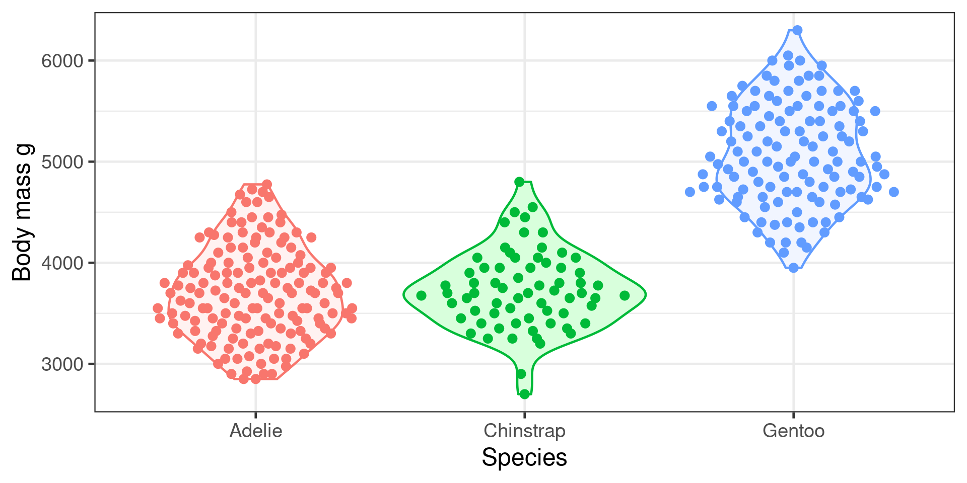
Does penguin body mass depend on species?
Predictor = species (categorical)
Response = body mass (continuous)
Hypotheses
\[H_0: \mu_{Adelie} = \mu_{Chinstrap} = \mu_{Gentoo}\] \(H_A\) At least two of the means differ
Fitting the model
Anova for categorical variables
Anova Table (Type II tests)

Response: body_mass_g
            Sum Sq  Df F value Pr(>F)
species   1.47e+08   2     344 <2e-16 ***
Residuals 7.24e+07 339
---
Signif. codes:  0 '***' 0.001 '**' 0.01 '*' 0.05 '.' 0.1 ' ' 1
At least two groups differ
summary for categorical variables
Call:
lm(formula = body_mass_g ~ species, data = penguins)

Residuals:
    Min      1Q  Median      3Q     Max
-1126.0  -333.1   -33.1   316.9  1224.0

Coefficients:
                 Estimate Std. Error t value Pr(>|t|)
(Intercept)        3700.7       37.6   98.37   <2e-16 ***
speciesChinstrap     32.4       67.5    0.48     0.63
speciesGentoo      1375.4       56.1   24.50   <2e-16 ***
---
Signif. codes:  0 '***' 0.001 '**' 0.01 '*' 0.05 '.' 0.1 ' ' 1

Residual standard error: 462 on 339 degrees of freedom
  (2 observations deleted due to missingness)
Multiple R-squared:  0.67,  Adjusted R-squared:  0.668
F-statistic:  344 on 2 and 339 DF,  p-value: <2e-16
Summary shows difference between
- Adelie and Chinstrap
- Adelie and Gentoo
Not between
- Chinstrap and Gentoo
Forcing the reference level
Very useful when you have a control
Multiple comparisons
- Don’t change the order of the levels of the predictor variable to compare all groups against each other
- use a post-hoc multiple comparisons test
     Simultaneous Tests for General Linear Hypotheses

Multiple Comparisons of Means: Tukey Contrasts


Fit: lm(formula = body_mass_g ~ species, data = penguins)

Linear Hypotheses:
                        Estimate Std. Error t value Pr(>|t|)
Chinstrap - Adelie == 0     32.4       67.5    0.48     0.88
Gentoo - Adelie == 0      1375.4       56.1   24.50   <1e-05 ***
Gentoo - Chinstrap == 0   1342.9       69.9   19.22   <1e-05 ***
---
Signif. codes:  0 '***' 0.001 '**' 0.01 '*' 0.05 '.' 0.1 ' ' 1
(Adjusted p values reported -- single-step method)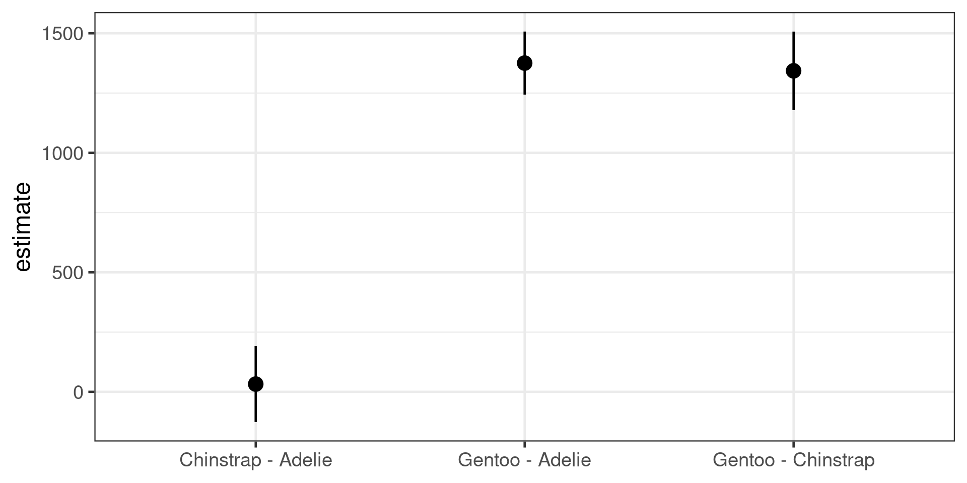
Assumptions of Least Squares
- The relationship between the response and the predictors is ~linear.
- The residuals have a mean of zero.
- The residuals have constant variance (not heteroscedastic).
- The residuals are independent (uncorrelated).
- The residuals are normally distributed.
Violation of assumptions cannot be detected using the t or F statistics or R2
Diagnostic plots
plot()base R diagnostic plotsautoplot()fromggfortify- same plots but prettiercheck_model()fromperformance- more diagnosticsDHARMapackage - very powerful diagnostics
performance
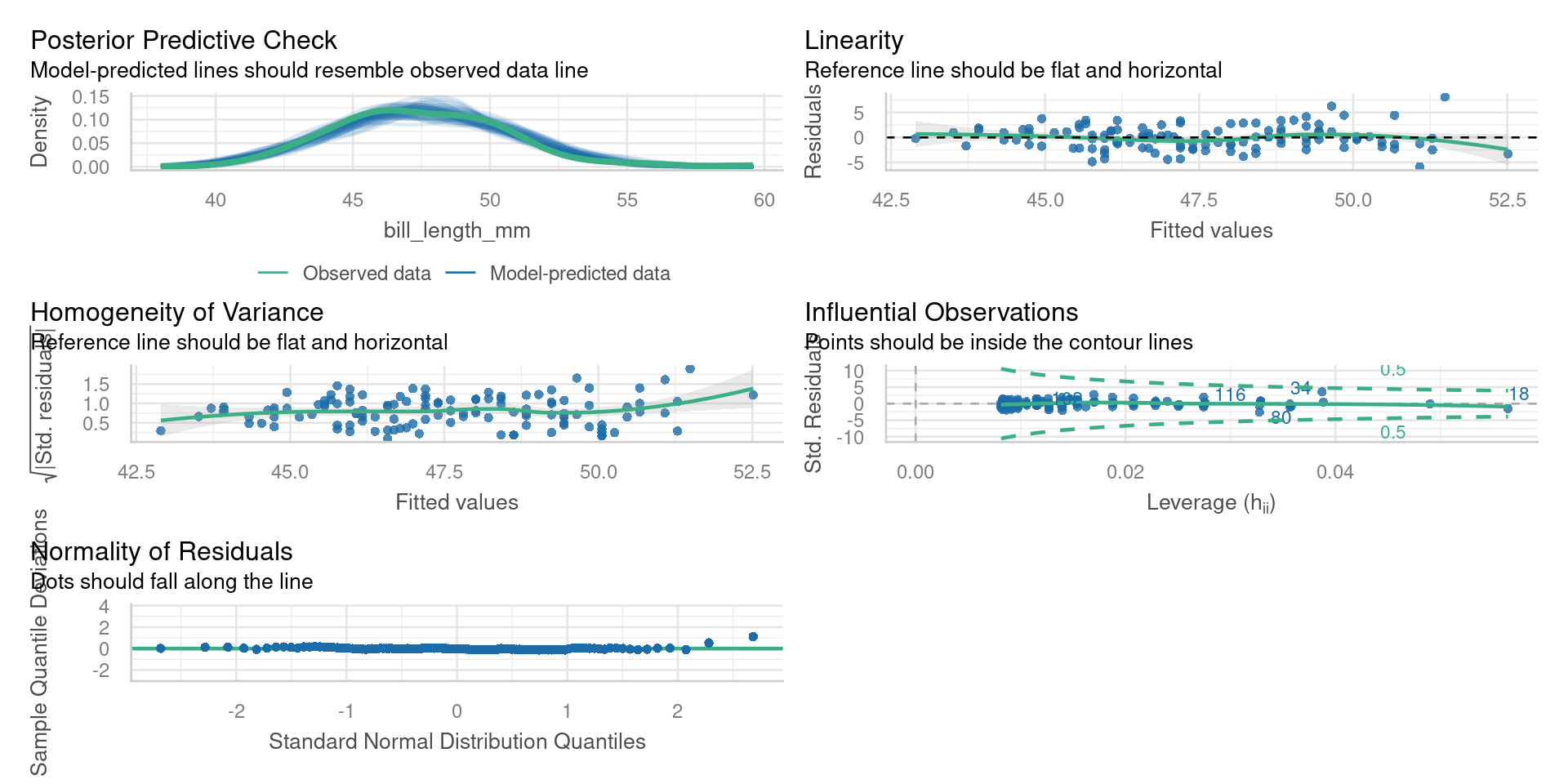
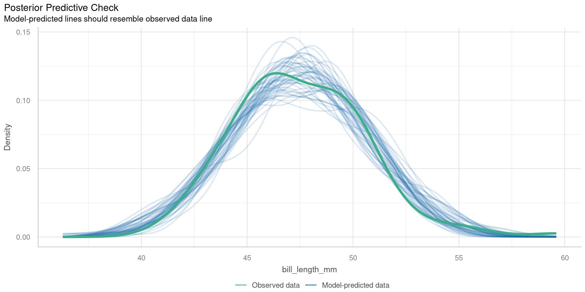
Posterior predictive checks
Check for systematic discrepancies between real and simulated data
- green - density of observed response
- blue - density of simulated response
Want green line to resemble blue lines
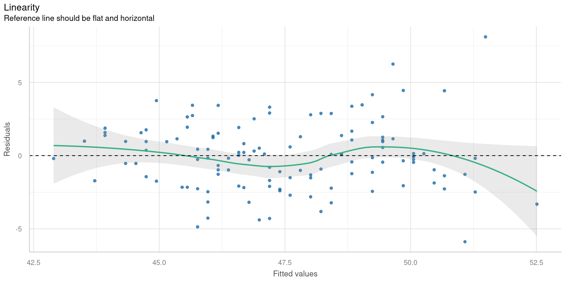
Residual vs fitted
Check for
- Outliers
- Variations in the mean residual
Want flat line
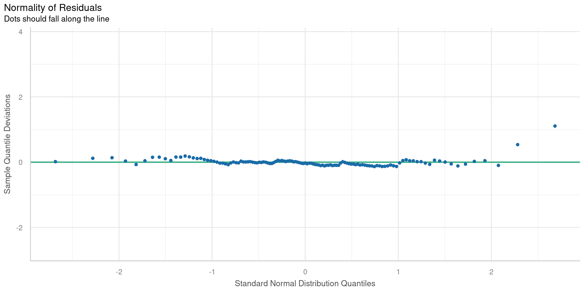
Quantile-quantile plot
QQ plots compare two samples to determine if they are from the same distribution.
Check for
- Non-normal distribution of the residuals
Points will lie on straight line if normally distributed
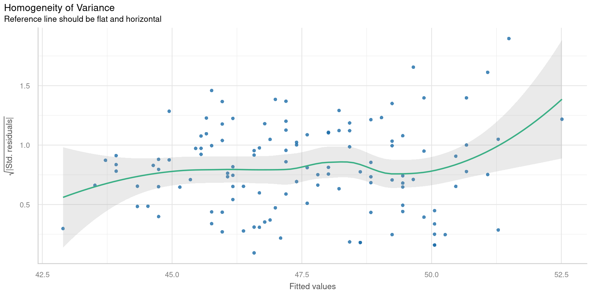
Scale-location plot
Square root of the absolute standardised residuals
Check for
- Unequal variance = Heteroscedasticity
Want flat line
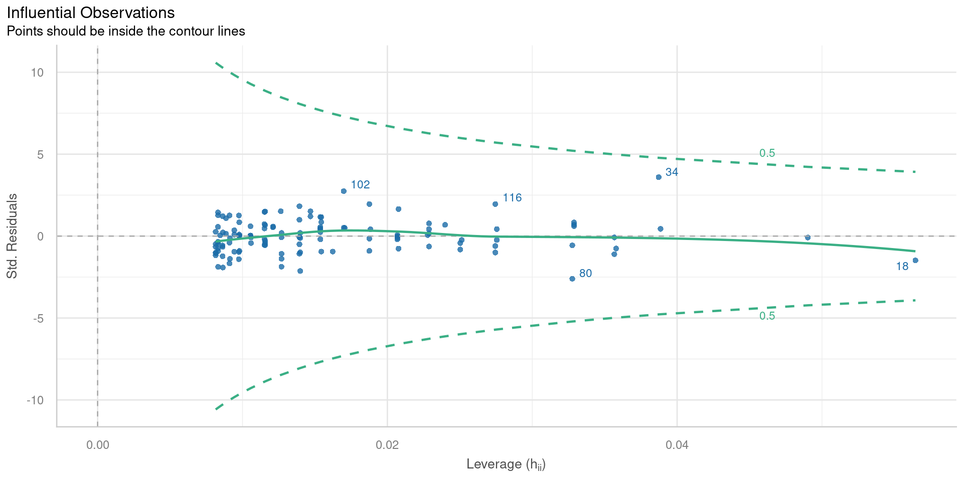
Residuals vs leverage
Plot of standardised residuals against leverage, with contours of Cooks distance
Observations with extreme leverage should be checked
Predictions
\[y = \beta_0+\beta_1x\]
Predict
    1     2     3     4     5     6     7     8     9    10    11    12    13
45.15 50.06 44.94 50.06 48.83 45.35 46.38 48.01 44.74 47.81 45.76 49.44 45.76
   14    15    16    17    18    19    20    21    22    23    24    25    26
50.67 43.92 50.67 43.72 52.51 46.38 48.63 50.06 47.19 44.74 47.40 47.19 47.60
   27    28    29    30    31    32    33    34    35    36    37    38    39
43.51 49.85 45.56 49.44 48.22 45.97 47.40 51.49 47.81 48.83 46.99 48.22 44.53
   40    41    42    43    44    45    46    47    48    49    50    51    52
48.63 42.90 50.06 44.33 46.17 49.44 46.78 43.92 48.83 47.60 48.42 46.58 48.42
   53    54    55    56    57    58    59    60    61    62    63    64    65
44.74 47.19 46.78 47.40 44.33 47.19 44.94 49.44 43.92 48.42 44.74 49.85 45.97
   66    67    68    69    70    71    72    73    74    75    76    77    78
50.06 45.76 50.47 45.97 49.44 46.17 47.19 47.60 48.01 45.97 50.47 45.56 51.28
   79    80    81    82    83    84    85    86    87    88    89    90    91
46.17 51.08 45.66 49.03 46.07 48.63 46.17 49.65 45.56 48.42 46.68 49.44 46.99
   92    93    94    95    96    97    98    99   100   101   102   103   104
48.83 46.17 49.85 46.58 48.01 46.89 46.68 45.66 48.22 46.58 49.65 47.09 49.24
  105   106   107   108   109   110   111   112   113   114   115   116   117
46.07 49.24 45.97 49.24 45.46 49.24 47.19 51.08 45.76 49.24 44.64 50.67 46.68
  118   119   121   122   123   124
51.28 46.89 46.58 50.26 48.01 48.83
Predict with new data
Predictions with standard errors
Uncertainty of the mean
Predictions with confidence interval
Often easier to use broom::augment()
Predictions interval
Where will a new observation probably be