4 Figures, tables and equations

4.1 Figures made in R

Plots can be included with a chunk that makes a figure with either base plot or ggplot.

If you make the plot with ggplot, remember to print it.

```{r}
#| label: histogram
#| fig-cap: "An embedded figure"
p <- ggplot(penguins, aes(x = bill_length_mm)) + 
  geom_histogram()
p # remember to print the plot
```

4.1.1 Figure chunk options

There are several useful chunk options for figures, including:

• fig-cap figure caption.
• fig-alt alternate text to improve accessibility
• fig-height figure height in inches (1 inch = 25.4 mm)
• fig-width figure width in inches

Exercise

The figure of height against treatment is missing a caption. Use code block options to give it an appropriate caption and alt-text.

Many journals require figures to be a specific size so they fit with the journal layout. For PLOSone, figures that fit in one column can be up to 13.2 cm (5.2 inches) wide. Use code block options to ensure that the figure would fit.

4.2 Embedding external images

In the visual editor, photographs and other figures that have been prepared outside of R can be included with the insert tool by typing “/” on a blank line and choosing “Figure/Image”. This will open an menu to get the path to the image and set the caption etc. Once you close the menu, you can set the figure size. This will generate a bit of markdown that looks like.

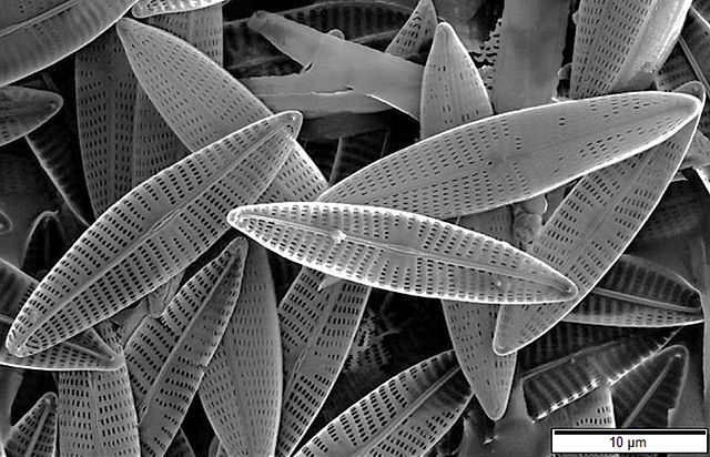![Marine diatoms](Pics/Marine_diatoms_SEM2.jpg){fig-alt="SEM photograph of marine diatoms" width="491"}

Marine diatoms

Alternatively, you can use knitr::include_graphics() in a regular code block.

knitr::include_graphics("Pics/Marine_diatoms_SEM2.jpg")

Figure 4.1: An embedded figure of diatoms

Use the out.width and out.height chunk options to set the display size of the figure.

4.3 Tables

You can make tables in markdown by hand (the / insert tool helps a lot), but it often so much easier to use R.

Simple tables can be made with the function knitr::kable. Several packages, including kableExtra and gt can make beautiful tables.

4.3.1 kable

knitr::kable(x = slice(penguins, 1:5), #the data for the table
             caption = "The top penguins" # the caption
)

Table 4.1: The top penguins

species	island	bill_length_mm	bill_depth_mm	flipper_length_mm	body_mass_g	sex	year
Adelie	Torgersen	39.1	18.7	181	3750	male	2007
Adelie	Torgersen	39.5	17.4	186	3800	female	2007
Adelie	Torgersen	40.3	18.0	195	3250	female	2007
Adelie	Torgersen	NA	NA	NA	NA	NA	2007
Adelie	Torgersen	36.7	19.3	193	3450	female	2007

4.3.2 gt

The gt package can make more elaborate tables than knitr::kable().

library(gt)
penguins |>
  slice(1:5) |> 
  gt(caption = "Basic gt table")

Table 4.2: Basic gt table

species	island	bill_length_mm	bill_depth_mm	flipper_length_mm	body_mass_g	sex	year
Adelie	Torgersen	39.1	18.7	181	3750	male	2007
Adelie	Torgersen	39.5	17.4	186	3800	female	2007
Adelie	Torgersen	40.3	18.0	195	3250	female	2007
Adelie	Torgersen	NA	NA	NA	NA	NA	2007
Adelie	Torgersen	36.7	19.3	193	3450	female	2007

penguins |>
  slice(1:5) |> 
  rename_with(str_to_sentence) |>
  gt(caption = "gt table with more features") |> 
  cols_label(Bill_length_mm = "Length mm",
             Bill_depth_mm  = "Depth mm",
             Flipper_length_mm = "Flipper length mm", 
             Body_mass_g = "Body mass g") |> 
  tab_spanner(label = "Bill", columns = c(Bill_length_mm, Bill_depth_mm)) |> 
  tab_spanner(label = "Body", columns = c(Flipper_length_mm, Body_mass_g)) 

Table 4.2: gt table with more features

Species	Island	Bill		Body		Sex	Year
		Length mm	Depth mm	Flipper length mm	Body mass g
Adelie	Torgersen	39.1	18.7	181	3750	male	2007
Adelie	Torgersen	39.5	17.4	186	3800	female	2007
Adelie	Torgersen	40.3	18.0	195	3250	female	2007
Adelie	Torgersen	NA	NA	NA	NA	NA	2007
Adelie	Torgersen	36.7	19.3	193	3450	female	2007

4.4 Number of decimal places

When reporting real numbers (i.e. numbers that have a decimal part), you need to decide how many digits to display. Be careful not to show spurious precision. You can use round() to remove unwanted decimals, or gt::fmt_number() to clean up one or more columns in a table. To control the default number of decimals across the whole document, use options(digits = 2) in the first chunk.

Exercise

Write a code block to make a table showing the mean leaf thickness and its standard deviation for each month.

Hint

sd() for standard deviation

group_by() and summarise() then use any of the table making functions.

4.5 Equations

Equations are embedded in a pair of dollar symbols. RStudio will show a preview of the equation as you type it. Equations are written with LaTeX notation.

What	How	Output
Lower-case Greek letters	$\sigma$	`$\sigma$`
Upper-Case Greek Letters	$\Sigma$	`$\Sigma$`
Subscript	$\beta_{0}$	`$\beta_{0}$`
Superscript	$\chi^{2}$	`$\chi^{2}$`
Fractions	$\frac{1}{2}$	`$\frac{1}{2}$`
Roots	$\sqrt{4} = 2$	`$\sqrt{4} = 2$`

Here is an example of using an inline equation.

The $\delta^{13}C$ value ...

The \(\delta^{13}C\) value …

A double dollar enclosure gives the equation its own line. For example, this is the equation of a standard deviation that uses several different elements.

$$SD = \sqrt{\frac{\sum_{i=1}^{n}{(x_i - \bar{x})^2}}{n-1}}$$

\[SD = \sqrt{\frac{\sum_{i=1}^{n}{(x_i - \bar{x})^2}}{n-1}}\]

When making a complex formula, build one element at a time, often starting in the middle, rather than trying to get it all working at once.

4.6 Chemistry

Equations are printed in an italic font, which is not great for chemical formulae. We can fix this with the \mathrm command which forces roman typeface.

Sulphate $\mathrm{SO_4^{2-}}$

Sulphate \(\mathrm{SO_4^{2-}}\)

$$\mathrm{CO_3^{2-} + H^+ \rightleftharpoons HCO_3^{2-}}$$

\[\mathrm{CO_3^{2-} + H^+ \rightleftharpoons HCO_3^{2-}}\]