3  Getting started with targets

In this chapter, you will

• learn the basic targets workflow
• build your own targets pipeline

3.1 Introduction to targets

Targets is a pipeline tool, which coordinates the different steps in data science in R. It manages the workflow, takes care of dependencies in the code and keeps track of outdated objects. Targets takes care of the cash.

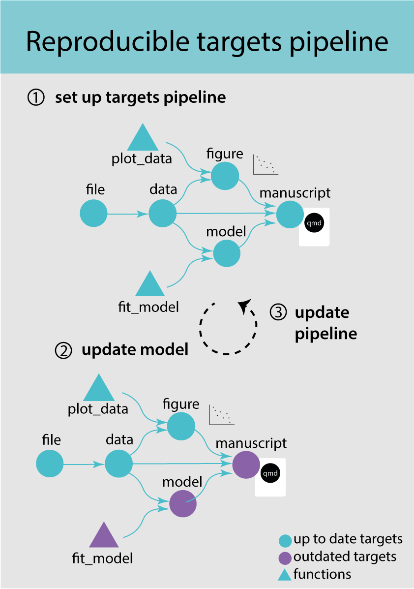
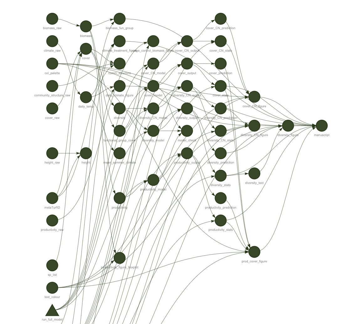
A targets pipeline consists of different steps, such as importing data, running an analysis or making a figure (Figure 3.1) (1). Each step in the pipeline is a target and can for example be a data frame, a model or a figure. A target is basically an R object and is created by a function. A pipeline has a main script that puts all the pieces of code together and takes care of dependencies and keeping track of changes.

This concept should sound familiar to you after reading the previous chapter on abstraction.

Definitions

• pipeline tool - coordinates different steps of data science
• target - an R object in memory
• function - self contained code that accomplish a specific task

When updating and rerunning one part of the code, targets will skip parts where the upstream code has not changed and are therefore still up to date (Figure 3.1) (2). Targets will only rerun the code that is outdated and ensures that your results always match the underlying code and maintains a reproducible workflow (3). It avoids unnecessary repetition and can save costly running time.

Figure 3.1: Reproducible targets pipeline.

When is targets useful?

• When the code has a long runtime because it is slow or complex. Targets avoids running code that up to date and allows for parallel processing.
• When the workflow has interconnected tasks with dependencies

3.2 The targets pipeline

3.2.1 The file structure

A target workflow has a specific file structure including R code, functions, qmd files, data and a _targets.R file (Figure 3.2). The _targets.R file is mandatory and the most important file defining the targets pipeline. This file lives at the root of the R project folder.

Figure 3.2: Minimal file structure of a target pipeline.

An R project will have many other files and it is recommended to keep code and data files in separate folders to keep the repository tidy. It is common to have one or several scripts that contain custom user-defined functions. These scripts should be stored in one folder. In this example we will call the folder R: R/functions.R.

To set up this file structure in an RStudio project, use the use_targets() function, which creates an initial _targets.R script with comments to help you populate the script.

Exercise

Go to the targets-workflow-svalbard Rstudio project and load the targets library library(targets). Then start to set up a targets pipeline by using the use_targets() function.

3.2.2 The _target.R file

The _targets.R file is the main script and configures and defines the pipeline. This file is mandatory and without it the targets pipeline will not work. When using the use_targets() function, it sets up the basic structure and comments to help fill out the rest (see below 👇) .

# Created by use_targets().
# Follow the comments below to fill in this target script.
# Then follow the manual to check and run the pipeline:
#   https://books.ropensci.org/targets/walkthrough.html#inspect-the-pipeline

# Load packages required to define the pipeline:
library(targets)
# library(tarchetypes) # Load other packages as needed.

# Set target options:
tar_option_set(
  packages = c("tibble") # Packages that your targets need for their tasks.
  # format = "qs", # Optionally set the default storage format. qs is fast.
  #
  # Pipelines that take a long time to run may benefit from
  # optional distributed computing. To use this capability
  # in tar_make(), supply a {crew} controller
  # as discussed at https://books.ropensci.org/targets/crew.html.
  # Choose a controller that suits your needs. For example, the following
  # sets a controller that scales up to a maximum of two workers
  # which run as local R processes. Each worker launches when there is work
  # to do and exits if 60 seconds pass with no tasks to run.
  #
  #   controller = crew::crew_controller_local(workers = 2, seconds_idle = 60)
  #
  # Alternatively, if you want workers to run on a high-performance computing
  # cluster, select a controller from the {crew.cluster} package.
  # For the cloud, see plugin packages like {crew.aws.batch}.
  # The following example is a controller for Sun Grid Engine (SGE).
  # 
  #   controller = crew.cluster::crew_controller_sge(
  #     # Number of workers that the pipeline can scale up to:
  #     workers = 10,
  #     # It is recommended to set an idle time so workers can shut themselves
  #     # down if they are not running tasks.
  #     seconds_idle = 120,
  #     # Many clusters install R as an environment module, and you can load it
  #     # with the script_lines argument. To select a specific verison of R,
  #     # you may need to include a version string, e.g. "module load R/4.3.2".
  #     # Check with your system administrator if you are unsure.
  #     script_lines = "module load R"
  #   )
  #
  # Set other options as needed.
)

# Run the R scripts in the R/ folder with your custom functions:
tar_source()
# tar_source("other_functions.R") # Source other scripts as needed.

# Replace the target list below with your own:
list(
  tar_target(
    name = data,
    command = tibble(x = rnorm(100), y = rnorm(100))
    # format = "qs" # Efficient storage for general data objects.
  ),
  tar_target(
    name = model,
    command = coefficients(lm(y ~ x, data = data))
  )
)

Exercise

Open the _targets.R in your repo and have a look at your _targets.R file.

The _targets.R file has four main components.

1. Load necessary R packages
2. Define settings
3. Source necessary functions
4. Write pipeline

Note that the file also contains other options which are optional. We will discuss the four main component step-by-step.

1. Load the necessary R packages to get the pipeline started. This will mainly be the targets and maybe the tarchetypes package.

The tarchetypes package contains helper functions and needs to be loaded if your pipeline contains a quarto file (see next chapter).

2. tar_option_set() sets all options such as load necessary packages or defining the output format. The argument package should have a list of all the required packages that are needed to run the pipeline. Note that targets needs to be loaded first and outside this function, otherwise the it cannot execute the tar_option_set() function.

The argument format let’s you define default storage format.

# Load packages required to define the pipeline:
library(targets)
# library(tarchetypes) # Load other packages as needed.

# Set target options:
tar_option_set(
  packages = c("tibble"), # packages that your targets need to run
  format = "rds" # default storage format
  # Set other options as needed.
)

Note that packages that are only used in a quarto file can be loaded directly in there and do not need to be loaded in the _targets.R file.

3. The function tar_source() will source all R scripts in the folder called R in the environment of the pipeline. It will by default search scripts in the folder called R. You can have the code in another folder and tell the function where to look for R srcipts tar_source("other_folder/functions.R") Importantly, the folder containing the code should be clean and only contain code that is used for the pipeline. Otherwise tar_source() will try to run other scripts in the folder.

# Run the R scripts in the R/ folder with your custom functions:
tar_source()

4. In the last section the pipeline is defined consisting of a list of targets. Each target is a step in the pipeline, for example importing data, run an analysis or make a figure and looks like a normal R object (e.g. tibble, vector, figure). Each target is declared by the tar_target() function and separated by a comma. The tar_target() needs two arguments: name defines the target name and command the code to produce the target. Usually the command is calling a custom function.

Here is a target that uses the function fit_model() that was created in the previous chapter to run a linear regression.

# fit model for plant height
list(
  tar_target(name = model,
             command = fit_model(data))
  )

Each target should have a unique name that can be called downstream in the pipeline. The order of the targets does not matter. The pipeline will figure out which targets depends on each other and run them in the right order.

Once the pipeline has run, the targets are stored.

Targets names

Targets names must be unique (no duplicates), should not start with a dot and the name should be meaningful (do not use my_variable).

Data files are special targets, because they also need the argument format to declare that this target is a file. Each time the pipeline is run, targetes will check if the file has been changed and if this is the case automatically import the data again the next time the pipeline is run.

list(
  tar_target(name = file,
             command = here::here("data/PFTC4_Svalbard_2018_Gradient_Traits.csv"),
             format = "file")
  )

How many targets should I make?

A target should do one thing only (e.g. make a figure) and if a functions gets too long, it can be split into nested sub-functions to make the code readable and easier to maintain. Keep the number of targets manageable, which means keep a balance between the amount of code that goes in one target and the number of targets.

3.2.3 Populate the _target.R file

Now we can populate the _targets.R file. We need to set the options, source the custom functions, and define the pipeline.

First, we need to add all R packages to the tar_option_set() function in the _targets.R file that are needed to run the pipeline.

Exercise

Add all the necessary R packages in tar_option_set() in the _targets.R file that are needed to run the pipeline.

# Set target options:
tar_option_set(
  packages = c("tidyverse") # packages that your targets need to run
)

The next step is to source all the functions. The tar_source() function in the _targets.R file already does this. But we are missing one last function to make the figure.

Exercise

Write a function that makes a figure showing leaf area in both gradients. Add this function to the function.R script and save the file.

The last step is to set up the targets pipeline.

Exercise

Define the data file

Add the dataset as data file in the _targets.R file. Save the file.

list(
  tar_target(name = file,
             command = path,
             format = "file")
  )

Exercise

Add other targets to the pipeline

Add four more targets to the pipeline that

• import the data

• clean the data

• run a linear regression

• and make a figure

The last three targets are calling custom functions from the functions.R file. The targets are separated by a comma. At the end save the file.

list(
  # data file
  tar_target(name = file,
             command = path,
             format = "file"),
  
  # import data
  tar_target(name = target1,
             command = function1),
  
  # clean data
  tar_target(name = target2,
             command = function2),
  
  ...
  
  )

Well done, you have just set up your first target pipeline. Have a treat 🥕!

3.2.4 Run the pipeline

Now we are ready to run the pipeline. Note that all R files that are used in the pipeline need to be saved before you run the pipeline. The function tar_make() runs the pipeline. This function looks for the _targets.R in the working directory and runs the pipeline. It makes sure the pipeline is run in the correct order.

When running the pipeline for the first time you will see a list of all the targets that are dispatched and completed (Figure 3.3).

Figure 3.3: R output after running the pipeline for the first time.

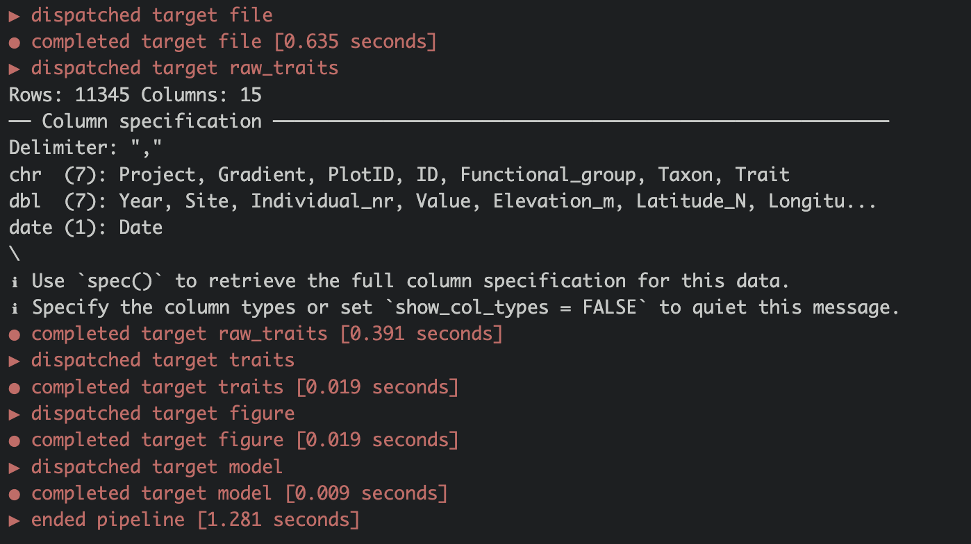
All targets are saved to the _targets/folder.

Exercise

Use tar_make() to run the pipeline. Hopefully, everything will run smoothly 🤞! If not check out the Trouble shooting section below.

Well done you have run your first targets pipeline. The tar_visnetwork() function shows the dependency graph of the pipeline and is a nice way of vizualizing the pipeline. Circles are targets, triangles functions, and the colour indicates if the targets are up to date or not.

Figure 3.4: Vizualise the targets pipeline.

Exercise

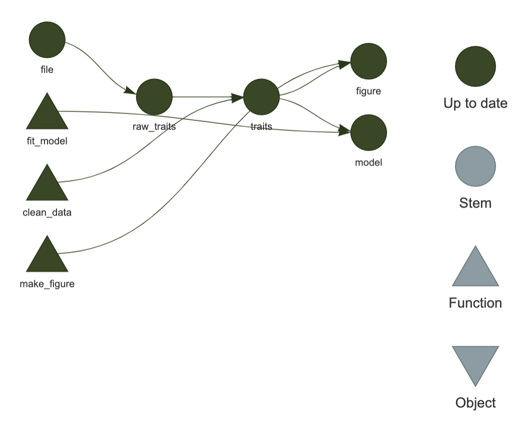
Run tar_visnetwork() to visualize your pipeline.

Once the pipeline has run, it will always skip the targets that have not changed and are up to date and only run the once that need updating. In the long run this will save a lot of computational time and is one of the big advantages of using targets pipelines.

Figure 3.5: R output after running the pipeline.

Exercise

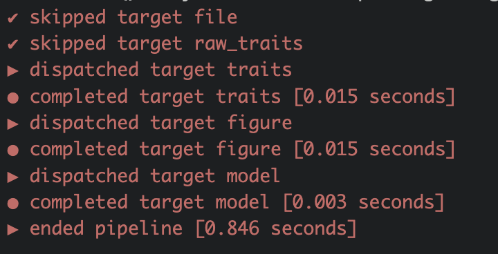
Change something in your pipeline. For example filter for a different species: bistorta vivipara. Save the script and run tar_visnetwork() to visualize which object are not up to date now.

Rerun the pipeline using tar_make().

And run tar_visnetwork() again to check if everything is up to date again.

3.2.5 Load targets

Each target can be loaded using tar_load() and the pipeline does not need rerunning each time before accessing the targets. This is a huge advantage of the targets pipeline and can save a lot of time.

tar_load(model)

To access all the targets at once use tar_load_everything(). In tar_load() you can also use tidy select commands to load specific targets, e.g. tar_load(starts_with("y"))

Exercise

Use tar_load() to load the target traits.

Run str(traits) to display the structure of the object traits.

Do it step-by-step

Targets plans can become huge and complex. Start small, create a few targets and functions and make the plan running. Then add new code in small steps and check regularly if the plan is still working This will help to understand and solve errors (see trouble shooting section).

Figure 3.6: Vizualisation of complex target pipeline.

3.3 Trouble shooting

3.3.1 Locate problem

Error messages in targets can be hard to understand and will look something like this:

Figure 3.7: Error in the pipeline.

You can see that the pipeline broke when running the target model. To learn more about the problem run the command targets::tar_meta(fields = error, complete_only = TRUE).

Figure 3.8: Find out more about a problem in the pipeline.

The R output now gives some more information about the problem. Here the argument response is missing.

If an error is difficult to understand use tar_load() to load one specific target or tar_load_everything() to load all targets. Then you can try to run different parts of the script to test where the code breaks.

Best practice is to run the pipeline regularly, which makes it easier locate where the error occurred.

3.3.2 Object not found

A common error is to call a target that does not exist. When running the pipeline this error will appear (Figure 3.9). This is usually if the name is spelled wrong or when using an old name.

Figure 3.9: Error message for missing object

3.3.3 Duplicate target

Another common mistake is to use the same name for two different targets (Figure 3.10). This is common when copy pasting code. Rename one of the objects and the problem is solved.

Figure 3.10: Error message for duplicate target.

3.3.4 Clean pipeline

Sometimes there are old targets in the pipeline that can cause problems. The tar_prune() function deletes data and metadata that are not used in the current pipeline anymore. The tar_delete() function deletes specific files that are stored in _targets/objects.

3.4 Resources

• The target manual contains everything you need to know and there is a large debugging section.
• Here is a large and working target plan
• A paper about pipelines: Brousil, M. R., Filazzola, A., Meyer, M. F., Sharma, S., & Hampton, S. E. (2023). Improving ecological data science with workflow management software. Methods in Ecology and Evolution. https://doi.org/10.1111/2041-210X.14113
• And finally, a short introduction to targets