
usethis::use_zip("biostats-r/biostats-data")11 Importing data in R
R can import data from files in many different formats. For example:
- csv files with the
readrpackage - excel files with the
readxlpackage - xlm files with the
xml2package - netcdf files with the
ncdf4package - shapefiles with the
sfpackage
In this chapter, you will learn how to import tabular data from an external text file as a tibble. We will use functions from the package readr which is part of the tidyverse package, so make sure that you have activated it with library(tidyverse).
NoteBefore we start
You must be familiar with tibbles and data types (such as numeric, character, etc).
You will need the following packages (in addition to those installed earlier)
here
You need to be working in an RStudio project (see Chapter 3).
NoteExercise
To import some data, you first need to download some.
We have made some files available which you can download with
When asked, agree to delete the zip file.
This will make a new directory called something like “biostats-r-biostats-data-9db4ebe/”. Rename this directory “data”. You can do this in the RStudio file tab.
11.1 What are tabular data?
Tabular data are data that is organized in the form of a table with rows and columns. A table often has a header, i.e. an additional row that displays variable names. Here is an example of a formatted table with header:
| month | temperature (Celsius) | precipitation (mm) | Wind (m/s) |
|---|---|---|---|
| January | -3.4 | 29.4 | 1.3 |
| February | -0.4 | 15.4 | 0.9 |
| March | -1.7 | 57.6 | 1.7 |
| april | 3.8 | 3.2 | 0.8 |
| May | 5.1 | 25.2 | 1.4 |
| June | 10.6 | 52.4 | 1.1 |
| July | 13.1 | 65.0 | 1.0 |
| August | 12.8 | 67.4 | 0.7 |
| September | 6.9 | 79.0 | 1.2 |
| October | 2.5 | 18.2 | 0.8 |
| November | -2.2 | 7.8 | 0.8 |
| December | 1.5 | 92.0 | 1.5 |
In this example, the table consists of 4 variables (columns) and 12 observations (rows) in addition to the header (top row). All cell contents are clearly delimited.
Below is an example of a non-tabular dataset. This dataset is a list of profiles with recurrent fields (Name, Position, Institution). Each profile contains three lines with a field:value pair.
Name: Aud Halbritter
Position: Researcher
Institution: UiB
-----------------------------
Name: Jonathan Soule
Position: Senior Engineer
Institution: UiB
-----------------------------
Name: Richard J. Telford
Position: Associate Professor
Institution: UiB
-----------------------------
11.2 File formats
Tabular data may be stored in files using various formats, spreadsheets, etc. The most common spreadsheets store data in their own, proprietary file format, e.g. MS Excel which produces .xls and .xlsx files. Such formats may be a limitation to data management in R. Simpler formats such as plain text files with .txt or .csv should always be preferred when saving data in spreadsheets.
11.3 Delimited files
One of the most common format for storing tabular data is plain text files with a delimiter between the columns. The delimiter is often a comma or a semi-colon, but other delimiters are possible including tabs.
Comma or semi-colon delimited files are known as CSV files, which stands for Comma-Separated Values, and often have a .csv extension. They may also have a .txt extension.
In a CSV-formatted file, the data is stored in a similar manner to this:
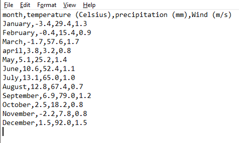
For information, this file matches the example in Table 11.1. Each line corresponds to a row in the table (including header) and cell contents are separated with a comma ,. Note that the period symbol . is used as decimal separator.
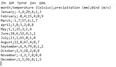
The use of commas in the CSV format is however not universal. Other symbols such as a semi-colon ; may be used as a delimiter. This is the case in several European countries where commas are decimal separator. Here is the same data set as above, this time in the European format:
11.4 Know your data!
There are several reasons why different symbols are used in CSV files. Among these reasons are:
- locale, i.e. the parameters that define the language and regional settings (currency, time and date, number format setting) in use on your machine,
- software-based preferences, the settings which are defined by default by the software that you have used to punch your data,
- user-based preferences, the settings that you choose when punching or saving data.
It is thus very important to know what your CSV file is made of. We therefore recommend to systematically inspect your data file before importing in R. One way to do it is to open the text file in a text editor (for example RStudio), or to read some of the file into R with read_lines('file.txt') (the n_max argument is useful if there is lots of data) and determine:
- which symbol is used as decimal separator (
,or.) - which symbol is used as delimiter (
,or;) - any extra lines of data that need removing
Here is our previous example:
read_lines("data/weather.csv") [1] "month,temperature (Celsius),precipitation (mm),Wind (m/s)"
[2] "January,-3.4,29.4,1.3"
[3] "February,-0.4,15.4,0.9"
[4] "March,-1.7,57.6,1.7"
[5] "april,3.8,3.2,0.8"
[6] "May,5.1,25.2,1.4"
[7] "June,10.6,52.4,1.1"
[8] "July,13.1,65.0,1.0"
[9] "August,12.8,67.4,0.7"
[10] "September,6.9,79.0,1.2"
[11] "October,2.5,18.2,0.8"
[12] "November,-2.2,7.8,0.8"
[13] "December,1.5,92.0,1.5" In this file, the decimal separator is . and the delimiter is ,.
11.5 Importing delimited files
We can import delimited files such as csv files with readr::read_delim(). read_delim() will import the data as a tibble.
Important
readr vs base R
Both readr and base R have functions for importing text files. They have different arguments, different defaults and behave differently, so be careful not to mix them up. readr functions have an underscore separating the words whereas base R uses a dot.
In the following example, we import the file weather.csv located in the subfolder data of the current RStudio project into the object weather.
library(tidyverse) # readr is part of the tidyverse
weather <- read_delim(file = "data/weather.csv")
Rows: 12 Columns: 4
── Column specification ────────────────────────────────────────────────────────
Delimiter: ","
chr (1): month
dbl (3): temperature (Celsius), precipitation (mm), Wind (m/s)
ℹ Use `spec()` to retrieve the full column specification for this data.
ℹ Specify the column types or set `show_col_types = FALSE` to quiet this message.When the function is executed, the console shows a short series of messages. In the frame above, the message Column specification tells you that the content of the column month has been recognized as of data type character, and that the three other columns have been recognized as double (which is similar to numeric).
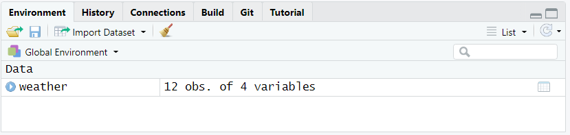
Now the tibble weather is available in R as you may see in the tab Environment (see Figure 11.2).
You can display the table as follows:
weather# A tibble: 12 × 4
month `temperature (Celsius)` `precipitation (mm)` `Wind (m/s)`
<chr> <dbl> <dbl> <dbl>
1 January -3.4 29.4 1.3
2 February -0.4 15.4 0.9
3 March -1.7 57.6 1.7
4 april 3.8 3.2 0.8
5 May 5.1 25.2 1.4
6 June 10.6 52.4 1.1
7 July 13.1 65 1
8 August 12.8 67.4 0.7
9 September 6.9 79 1.2
10 October 2.5 18.2 0.8
11 November -2.2 7.8 0.8
12 December 1.5 92 1.5
TipRemember to assign!
If you don’t assign (<-) the imported data to a name, the tibble will be printed to the screen and then lost.
11.5.1 File paths
The first argument to read_delim() is file. This wants the location of the file on your computer. Before we can import a file, we have to find it!
You might be tempted to write the absolute path to the file, something like:
"c:/user/bad13/documents/project/my_file.csv"This would be a bad idea. Why? Because this path only works on your current computer (provided you don’t move the file). This code won’t work for anyone else, so you cannot share the code with your supervisor and have them run it, nor archive it with a manuscript. The code is not reproducible.
Much better is to a path relative to your RStudio project (remember to use an RStudio project - for more info about them, read Chapter 3). If the contents of your RStudio project looked like this
.
├── R
│   ├── 01_import.R
│   └── 02_analyse.R
├── data
│   ├── 2022-3-24_lake-tilo-chemistry.csv
│   ├── 2022-3-24_lake-tilo-diatoms.csv
│   └── 2022-8-15_lake-tilo-diatoms.csv
├── my_project.Rproj
├── output
│   └── manuscript.pdf
└── quarto
    ├── manuscript.qmd
    └── references.bib
Now we could use
"data/2022-3-24_lake-tilo-chemistry.csv"to access the chemistry data. If we move the RStudio project to a different location on your computer, or another computer, the code will still work. You don’t even need to type the full name: just type the quote marks and a few characters and autocomplete will start making suggestions.
There is still a problem though. When we use a quarto document, the working directory is the directory where the quarto document is stored. This can cause some confusion, which we can avoid if we use the here package to find the RStudio project root.
Our import code would now look like this
library("here")
weather <- read_delim(file = here("data/weather.csv"))
Using here is highly recommended.
ImportantForward slashes and backslashes
Remember to use forward slashes / to separate directories in the path. If you use back slashes \, you will get an error as these are used to escape the following character (e.g., \t is a tab). If you really want back slashes, use two of them \\ as the first will escape the second. If you let autocomplete fill in your path, it will do it correctly
11.5.2 Delimiters
The second argument to read_delim() is the column delimiter delim.
It used to be very important to specify the delimiter (or choose a function such as read_csv() that had it set by default), but, after a recent update, read_delim() will guess what the delimiter is and we only need to specify it if it gets it wrong.
NoteExercise
Import the “weather.csv” data into R and assign it to an name.
11.5.3 Review the imported data
Once you have imported the data, it is important to inspect it to check that everything has worked as expected.
- does it have the correct number of columns (may indicate problems with the delimiter)
- are the columns the expected type
- are the values correct.
To do this, we can print the object or View() it. We can also get details of the column specification
spec(weather)cols(
month = col_character(),
`temperature (Celsius)` = col_double(),
`precipitation (mm)` = col_double(),
`Wind (m/s)` = col_double()
)Any parsing problems (for example if there text in a column that should be numeric) will be shown with problems()
problems(weather)# A tibble: 0 × 5
# ℹ 5 variables: row <int>, col <int>, expected <chr>, actual <chr>, file <chr>Here, there are no parsing problems so we get a tibble with zero rows.
Let’s try another example. File weather2.csv has semi-colons as delimiters.
weather2 <- read_delim(file = "data/weather2.csv")Rows: 12 Columns: 4
── Column specification ────────────────────────────────────────────────────────
Delimiter: ";"
chr (2): month, Wind (m/s)
num (2): temperature (Celsius), precipitation (mm)
ℹ Use `spec()` to retrieve the full column specification for this data.
ℹ Specify the column types or set `show_col_types = FALSE` to quiet this message.spec(weather)cols(
month = col_character(),
`temperature (Celsius)` = col_double(),
`precipitation (mm)` = col_double(),
`Wind (m/s)` = col_double()
)Here, the message Column specification tells you that the content of the columns month and Wind (m/s) has been recognized as of data type character, and that the two other columns have been recognized as number. While read_delim() got things right about the number of variables, something went wrong with the variables as we could expect Wind (m/s) to be recognized as double. To find out about this issue we need to review the imported data in the object weather2 and compare it to the original file weather2.csv.
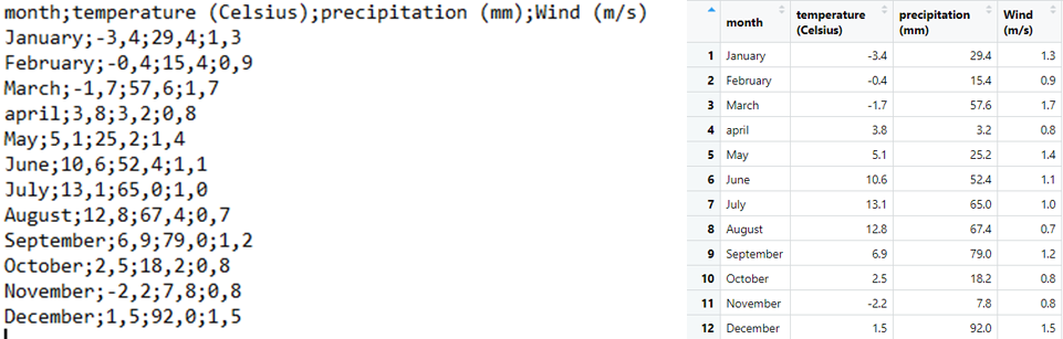
The example above shows the importance of carefully verifying that the imported data in R matches the original data set. The following figure compares the content of the file weather2.csv (Figure 11.3 left) to the content of the object weather2 (Figure 11.3 right):

Looking at the rows in both pictures, one can understand that all commas have simply been ignored, excepted those in the last column. To solve that issue, you must impose the separator using locale = locale(decimal_mark = ","):
weather3 <- read_delim(
  file = "data/weather2.csv",
  locale = locale(decimal_mark = ",")
)
Rows: 12 Columns: 4
── Column specification ────────────────────────────────────────────────────────
Delimiter: ";"
chr (1): month
dbl (3): temperature (Celsius), precipitation (mm), Wind (m/s)
ℹ Use `spec()` to retrieve the full column specification for this data.
ℹ Specify the column types or set `show_col_types = FALSE` to quiet this message.The last column is now recognized as double and the data in the object weather3 matches the data in the file:
ImportantDecimal seperators
While readr can guess the column delimiter, it cannot guess the decimal separator. The English/American standard is to use “.” as the separator. In Norway it is common to use a comma as the decimal separator (but “.” are also common). If you don’t specify the decimal separator, readr assumes that the comma is a thousand separator and ignores it. Then the values can be 10x higher than expected.
11.5.4 read_csv2()
A shortcut for files with a “;” as the column delimiter and commas as the decimal separator is read_csv2().
weather_csv2 <- read_csv2(file = "data/weather2.csv")ℹ Using "','" as decimal and "'.'" as grouping mark. Use `read_delim()` for more control.Rows: 12 Columns: 4
── Column specification ────────────────────────────────────────────────────────
Delimiter: ";"
chr (1): month
dbl (3): temperature (Celsius), precipitation (mm), Wind (m/s)
ℹ Use `spec()` to retrieve the full column specification for this data.
ℹ Specify the column types or set `show_col_types = FALSE` to quiet this message.Note the message above Column specification that indicates which symbols read_csv2() has considered when importing the data. The resulting tibble looks correct:
weather_csv2# A tibble: 12 × 4
month `temperature (Celsius)` `precipitation (mm)` `Wind (m/s)`
<chr> <dbl> <dbl> <dbl>
1 January -3.4 29.4 1.3
2 February -0.4 15.4 0.9
3 March -1.7 57.6 1.7
4 april 3.8 3.2 0.8
5 May 5.1 25.2 1.4
6 June 10.6 52.4 1.1
7 July 13.1 65 1
8 August 12.8 67.4 0.7
9 September 6.9 79 1.2
10 October 2.5 18.2 0.8
11 November -2.2 7.8 0.8
12 December 1.5 92 1.5
NoteExercise
Import the file weather2.csv. Make sure it has imported correctly.
11.5.5 Useful arguments
read_delim() and the other functions discussed above have a multitude of arguments that allow for adjusting the way data is read and displayed. Here we review a handful of them.
11.5.5.1 n_max
n_max sets a limit to the number of observations to be read. Note that n_max does not consider the first row (header) of the data file as an observation.
weather <- read_delim(
  file = "data/weather.csv",
  n_max = 6
)weather# A tibble: 6 × 4
month `temperature (Celsius)` `precipitation (mm)` `Wind (m/s)`
<chr> <dbl> <dbl> <dbl>
1 January -3.4 29.4 1.3
2 February -0.4 15.4 0.9
3 March -1.7 57.6 1.7
4 april 3.8 3.2 0.8
5 May 5.1 25.2 1.4
6 June 10.6 52.4 1.111.5.5.2 skip
The argument skip may be used to skip rows when reading the data file.
Be aware that:
- the header in the original data file counts as one row,
- the first row that comes after those which have been skipped becomes the header for the resulting tibble.
In the following example, we read the data file weather.csv and skip the first row:
weather <- read_delim(
  file = "data/weather.csv",
  skip = 1
)weather# A tibble: 11 × 4
January `-3.4` `29.4` `1.3`
<chr> <dbl> <dbl> <dbl>
1 February -0.4 15.4 0.9
2 March -1.7 57.6 1.7
3 april 3.8 3.2 0.8
4 May 5.1 25.2 1.4
5 June 10.6 52.4 1.1
6 July 13.1 65 1
7 August 12.8 67.4 0.7
8 September 6.9 79 1.2
9 October 2.5 18.2 0.8
10 November -2.2 7.8 0.8
11 December 1.5 92 1.5As expected, the first row (with the header) is skipped, and the data from the observation January have become the header of the tibble. The argument col_names() introduced below will be useful for solving this issue.
11.5.5.3 col_names
The argument col_names may be used to define the name of the variables/columns of the tibble.
col_names = may also be followed by the actual variable names that you want to use. In that case, write col_names = c() and list the names between the parentheses. Be aware that the first row of the original data file, which would have been the column names, will become the first row of the resulting tibble. This means that if you want to replace existing names, you should also use the skip argument.
Here is an example:
weather <- read_delim(
  file = "data/weather.csv",
  skip = 1,
  col_names = c("Month", "Temp", "Precip", "Wind")
)
weather
# A tibble: 12 × 4
Month Temp Precip Wind
<chr> <dbl> <dbl> <dbl>
1 January -3.4 29.4 1.3
2 February -0.4 15.4 0.9
3 March -1.7 57.6 1.7
4 april 3.8 3.2 0.8
5 May 5.1 25.2 1.4
6 June 10.6 52.4 1.1
7 July 13.1 65 1
8 August 12.8 67.4 0.7
9 September 6.9 79 1.2
10 October 2.5 18.2 0.8
11 November -2.2 7.8 0.8
12 December 1.5 92 1.5If lots of column names are badly formatted, it may be easier to use janitor::clean_names() to improve them.
weather <- read_delim(file = "data/weather.csv") |>
  janitor::clean_names()
weather
# A tibble: 12 × 4
month temperature_celsius precipitation_mm wind_m_s
<chr> <dbl> <dbl> <dbl>
1 January -3.4 29.4 1.3
2 February -0.4 15.4 0.9
3 March -1.7 57.6 1.7
4 april 3.8 3.2 0.8
5 May 5.1 25.2 1.4
6 June 10.6 52.4 1.1
7 July 13.1 65 1
8 August 12.8 67.4 0.7
9 September 6.9 79 1.2
10 October 2.5 18.2 0.8
11 November -2.2 7.8 0.8
12 December 1.5 92 1.511.5.5.4 col_types
The argument col_types may be used to modify the data type of the variables. This is useful for example when you need to set a variable as factor whereas R has defined it as character. Here is an example with three simple variables.
counts <- read_delim(file = "data/groups.csv")Rows: 9 Columns: 3
── Column specification ────────────────────────────────────────────────────────
Delimiter: ","
chr (1): group
dbl (2): ID, count
ℹ Use `spec()` to retrieve the full column specification for this data.
ℹ Specify the column types or set `show_col_types = FALSE` to quiet this message.As the message clearly indicates, the first and last variables are recognized as double (i.e. numeric) while the second one is recognized as character. The tibble in the object counts displays as follows:
counts# A tibble: 9 × 3
ID group count
<dbl> <chr> <dbl>
1 1 A 5
2 2 A 3
3 3 A 2
4 4 B 4
5 5 B 5
6 6 B 8
7 7 C 1
8 8 C 2
9 9 C 9Let’s use col_types = cols() to manually set the data types to double, factor and integer, respectively.
counts <- read_delim(
  file = "data/groups.csv",
  col_types = cols(col_double(), col_factor(), col_integer())
)
Now the tibble displays like this, with the correct data types for each column:
counts# A tibble: 9 × 3
ID group count
<dbl> <fct> <int>
1 1 A 5
2 2 A 3
3 3 A 2
4 4 B 4
5 5 B 5
6 6 B 8
7 7 C 1
8 8 C 2
9 9 C 9If you only need to modify one or a few variables, you must name it/them when writing the code:
counts <- read_delim(
  file = "data/groups.csv",
  col_types = cols(group = col_factor())
)
The tibble displays like this:
counts# A tibble: 9 × 3
ID group count
<dbl> <fct> <dbl>
1 1 A 5
2 2 A 3
3 3 A 2
4 4 B 4
5 5 B 5
6 6 B 8
7 7 C 1
8 8 C 2
9 9 C 9col_types is particularly useful when importing tabular data that includes formatted dates. Dates are usually recognized as character when their format does not match the expected format set as default (locale, etc). In the following example, dates entered as yyyy-mm-dd in the last column are recognized as of type date:
countsdates <- read_delim(file = "data/groups-dates1.csv")Rows: 9 Columns: 4
── Column specification ────────────────────────────────────────────────────────
Delimiter: ","
chr (1): group
dbl (2): ID, count
date (1): date
ℹ Use `spec()` to retrieve the full column specification for this data.
ℹ Specify the column types or set `show_col_types = FALSE` to quiet this message.However, in the example below, dates entered as dd-mm-yyyy are converted to character:
countsdates <- read_delim(file = "data/groups-dates2.csv")Rows: 9 Columns: 4
── Column specification ────────────────────────────────────────────────────────
Delimiter: ","
chr (2): group, date
dbl (2): ID, count
ℹ Use `spec()` to retrieve the full column specification for this data.
ℹ Specify the column types or set `show_col_types = FALSE` to quiet this message.To solve this issue, add the function col_date() in cols() to help R understand how dates are formatted and shall be read.
countsdates <- read_delim(
  file = "data/groups-dates2.csv",
  col_types = cols(date = col_date("%d-%m-%Y"))
)
The result is the following tibble now correctly formatted:
countsdates# A tibble: 9 × 4
ID group count date
<dbl> <chr> <dbl> <date>
1 1 A 5 2021-03-01
2 2 A 3 2021-03-02
3 3 A 2 2021-03-03
4 4 B 4 2021-03-01
5 5 B 5 2021-03-02
6 6 B 8 2021-03-03
7 7 C 1 2021-03-01
8 8 C 2 2021-03-02
9 9 C 9 2021-03-03You will find the whole list of cols() parameters for col_types here.
NoteExercise
Import the data from “biomass2015_H.csv”. These data are plant biomass data from an alpine grassland near Mt Gonga, China.
TipVery large files
readr imports objects into the computers memory. This is fine for most datasets. But very large datasets (gigabytes) - will not fit into memory and another solution is needed. We can use apache arrow with the arrow package or duckDB with duckplyr. Both can work with dplyr functions to process large datasets efficiently.
11.5.6 White space delimited files
Some files have white space separating the columns. If a single tab is used then read_delim() will automatically detect it and work correctly. Sometimes multiple spaces are used so the columns line up, making the text file easy for humans to read. read_delim() will not work with these files as it expects a single delimiter. Instead we can use read_table(), shown here with some test data.
read_table(" Species   Value
            Navicula       1
            Cymbella       2")
# A tibble: 2 × 2
Species Value
<chr> <dbl>
1 Navicula 1
2 Cymbella 2Another type of data you will sometimes see is the fixed width format. There are no delimiters, but each field has the same position in each row. These files can be imported with read_fwf(). Determining the position of each column can be painful unless you have good metadata.
NoteExercise
Import part “3a. Clegg et al. 2011 Hudson Lake Midge Temperature Data” from “alaska2011midge-t.txt”
Hint
skip and n_max argument can be useful.
TipReading multiple files
If you want to read many files with the same structure, you can supply read_delim() with a vector of files names.
# get a vector of files
files <- list.files(path = "data/", pattern = "csv")
files
#> file1.csv file2.csv

# read them in at once
# record paths in a column called filename
read_csv(files, id = "filename")
#> # A tibble: 4 × 3
#>   filename      x     y
#>   <chr>     <dbl> <dbl>
#> 1 file1.csv     1     2
#> 2 file1.csv     3     4
#> 3 file2.csv     5     6
#> 4 file2.csv     7     8
If the files do not have identical structures, perhaps one of the files has text where it should have a number, you either have to use the col_types argument to convert everything to the same format, or iterate (Chapter 16) over the files to import and fix them.
11.6 Excel files
Even though we don’t recommend you use Excel files for your own data, you need to know how to import such data as you may be given Excel files for find them in a data repository. To make your analysis reproducible, it is important to keep the files in their original format rather than converting them to CSV so that all the processing is done with code.
Excel files can be imported with the readxl package which is installed with tidyverse but not loaded until you run library(readxl). The function read_excel() will import the data; it can be worth using excel_sheets() first to check the names of the sheets.
library(readxl)
excel_sheets(path = "data/biomass2015.xls")
biomass_l <- read_excel(path = "data/biomass2015.xls", sheet = "Site L")
Many of the arguments for skipping rows at the start of the file, enforcing column types, etc, are similar to those in readr::read_delim()
ImportantSetting the locale on windows computers
The locale captures the defaults that vary between countries. If you are using a windows computer, the locale may not have been set correctly. This would cause the next exercise to fail, and any text with the Norwegian letters “å”, “ø” and “æ” or other diacritics.
Check if there is a problem by running
If this returns “C”, then you have a problem. To see the problem, run "å" (with quotes) in the console.
We can fix the problem permanently by editing the .rprofile file with instructions to set the locale correctly. To do this, run
usethis::edit_r_profile()This will create and open a .rprofile file. Now add the following line to the file, save it, and restart R (Session > Restart R).
Sys.setlocale(locale = "Norwegian.UTF-8")Other locale languages are avaliable, but always use “UTF-8” character encoding.
NoteExercise
Import the biomass data from Site A from biomass2015.xls
NoteFurther Reading
You may find the following links useful:
Contributors
- Jonathan Soulé
- Aud Halbritter
- Richard Telford