---
editor: visual
execute:
message: false
---
# Making maps in R {#sec-map-making}
```{r}
#| label: tidyverse
#| include: false
library(tidyverse)
library(patchwork)
source("R/setup.R")
```
Biologists need almost as many maps as geographers, perhaps to show where our field sites are, the range of a species, or the migration path of a bird.
Typically, the data we want to show is added to a base map.
These can be added to different types of base map
- vector map showing the coastline, and perhaps political borders, rivers and other features
- A map made of downloaded tiles (similar to how Google maps works)
::: callout-tip
## Terminology
Small scale vs large scale?
The terminology is confusing!
Map scales are given as a ratio.
A world map might have a scale of 1:100000000.
1 cm on the map represents 100000000 cm on the ground - a ratio of 1/100000000.
A small number hence a small-scale map.
Conversely, a map of a city might have a scale of 1:25000.
1 cm on the map represents 25000 cm on the ground - a ratio of 1/25000.
A large number hence a large-scale map.
Large-scale maps are usually high resolution and cover a small spatial extent.
:::
## Vector base maps
### `rnaturalearth`
The `rnaturalearth` package makes [Natural Earth](http://www.naturalearthdata.com/) data available.
Natural Earth [features include](https://www.naturalearthdata.com/features/) coastlines, rivers, bathymetry, political borders, roads and railways at scales 1:10m, 1:50m, and 1:110 million.
The low-resolution (1:110 million) coastline and country data, suitable for world maps, are included in the `rnaturalearth` package.
The `rnaturalearthdata` package, also on CRAN, contains medium-resolution data.
High-resolution (1:10 million) data are in the `rnaturalearthhires` package, instructions for installing this are below.
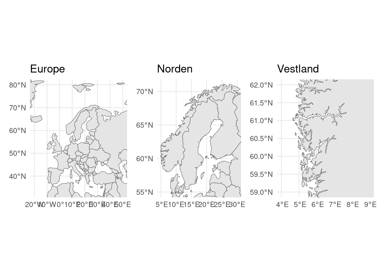
```{r}
#| label: rnaturalearth
#| results: hide
#| fig-alt: Maps at different scales
#| message: false
library(rnaturalearth)

world <- ne_countries(scale = 110)
small_scale_map <- ggplot() +
  geom_sf(data = world) +
  coord_sf(xlim = c(-20, 50), ylim = c(33, 80)) +
  ggtitle("Europe")

europe <- ne_countries(scale = 50, continent = "Europe")
medium_scale_map <- ggplot() +
  geom_sf(data = europe) +
  coord_sf(xlim = c(5, 30), ylim = c(55, 71)) +
  ggtitle("Norden")

# Need extra package for high resolution data
# install.packages("rnaturalearthhires", repos = "https://ropensci.r-universe.dev")

norway <- ne_countries(scale = 10, country = "Norway")

large_scale_map <- ggplot() +
  geom_sf(data = norway) +
  coord_sf(xlim = c(4, 9), ylim = c(59, 62)) +
  ggtitle("Vestland")

# combine maps with patchwork
library(patchwork)
small_scale_map + medium_scale_map + large_scale_map
```
`coord_sf()` is used to show only part of the map.
::: callout-tip
## `sf` and `sp` packages
`sf` and `sp` are both packages for geospatial data.
`sf` is the newer package that supports the "simple features" standard and is what I strongly recommend.
:::
::: {.callout-tip collapse="true"}
## Rivers and lakes and other Natural Earth data
Sometimes the coastline and national borders are sufficient.
Sometimes they aren't very informative and you want to add more features, such as rivers, lakes and cities.
This can be done with data from [Natural Earth](http://www.naturalearthdata.com/) (or other sources).
Natural Earth datasets can be downloaded directly from the [website](https://www.naturalearthdata.com/downloads/) or with `ne_download()`
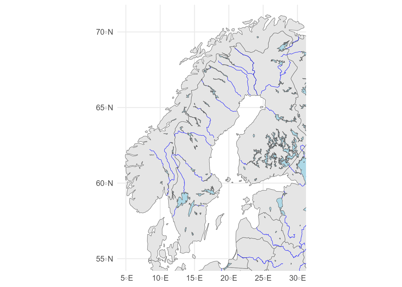
```{r}
#| label: fig-lakes-rivers
#| fig-cap: Lakes and rivers
#| fig-alt: Map showing lakes and rivers
#| message: false
#| results: hide
# download if needed
if (!file.exists("maps/ne_10m_rivers_europe.shp")) {
  ne_download(
    scale = 10, type = "rivers_lake_centerlines", category = "physical",
    destdir = "maps/", load = FALSE
  ) # major rivers
  ne_download(
    scale = 10, type = "lakes", category = "physical",
    destdir = "maps/", load = FALSE
  ) # major lakes
}

rivers <- ne_load(scale = 10, type = "rivers_lake_centerlines", destdir = "maps")
lakes <- ne_load(scale = 10, type = "lakes", destdir = "maps")

ggplot() +
  geom_sf(data = europe) +
  geom_sf(data = rivers, colour = "blue", linewidth = 0.2) +
  geom_sf(data = lakes, fill = "lightblue") +
  coord_sf(xlim = c(5, 30), ylim = c(55, 71))
```
Extra rivers and lakes for Europe and N.
America are available from Natural Earth, but for a large-scale map, other data sets may be better.
:::
### `ggOceanMaps`
`ggOceanMaps` is, as the name suggests, focused on ocean map, with coastlines, bathymetry and also glaciers.
The `ggOceanMaps` package includes some data, but high resolution data is downloaded when needed.
To avoid repeatedly downloading the same data, open the .Rprofile file by running
```{r}
#| label: setup-ggOceanMapsData
#| eval: false
usethis::edit_r_profile()
```
and add
```{r}
#| label: rprofile
#| eval: false
.ggOceanMapsenv <- new.env()
.ggOceanMapsenv$datapath <- "~/ggOceanMapsLargeData"
# you can use a different directory if you want.
# This one should work on any computer
```
Save the file and restart R (Session \> Restart R).
Now `ggOceanMaps` is ready to use.
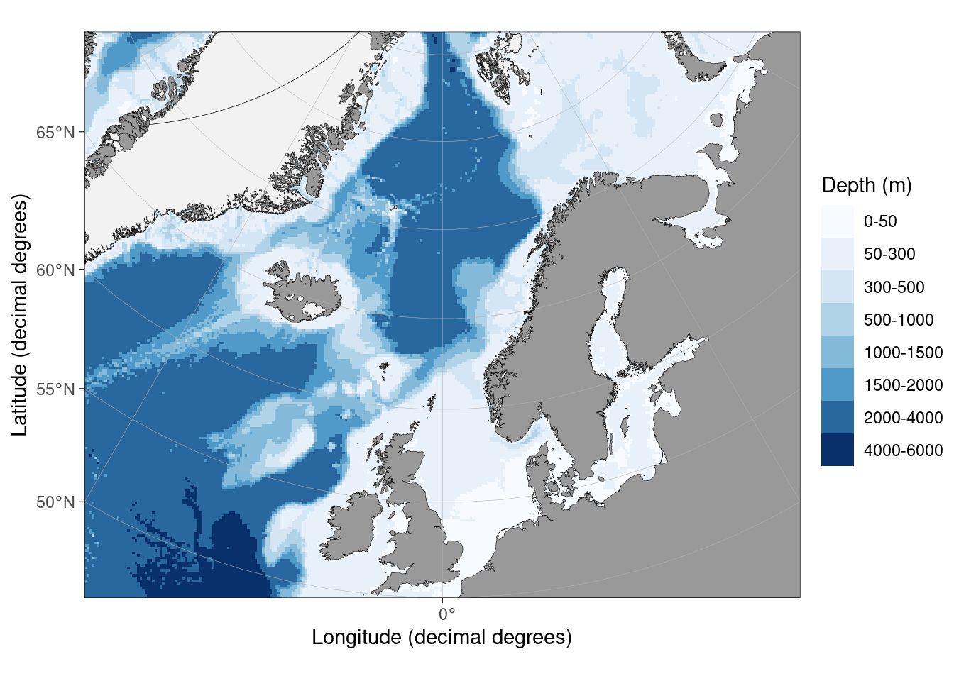
```{r}
#| label: ggOceanMaps
#| message: false
#| fig-alt: Base map from ggOceanMaps
library(ggOceanMaps)
# limits are given longitude min/max, latitude min/max
basemap(
  limits = c(-30, 30, 50, 80),
  bathymetry = TRUE,
  glaciers = TRUE
)
```
::: callout-note
## Exercise
Make a map of Svalbard using either `rnaturalearth` or `ggOceanMaps`.
:::
### Other vector files
The maps in `rnaturalearth` and `ggOceanMaps` are good and the global and regional scale, but lack resolution for local scale maps, and may lack features we are interested in.
For such maps we need to find alternative resources.
These could be a shapefile, GeoJSON or GeoPackage file, all of which can be imported with `sf::st_read()`.
::: callout-tip
## Shapefiles
A "shapefile" is not one file but collection of several files in the same directory, only of which has the extension ".shp".
:::
This is a map of the fylke of Norway.
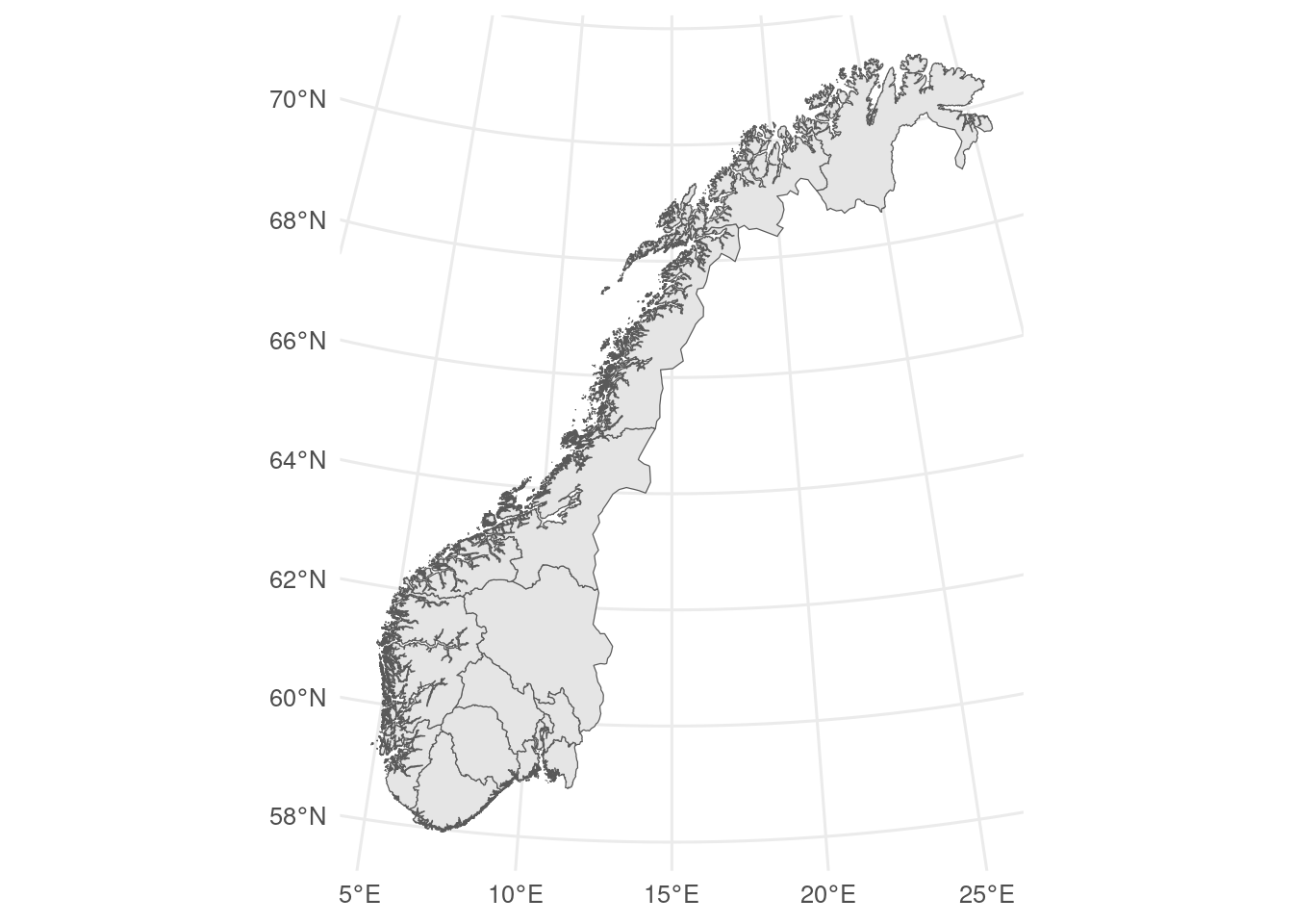
```{r}
#| label: fylker
#| fig-alt: Map showing fylke
#| results: hide
#| message: false
library(sf)

# https://kartkatalog.geonorge.no/metadata/norske-fylker-og-kommuner-illustrasjonsdata-2024-klippet-etter-kyst/a9c64d66-f484-4a8f-a7b4-723fdaa578d3

fylker <- st_read("data/Fylker.geojson")

ggplot(fylker) +
  geom_sf()
```
::: {.callout-tip collapse="true"}
## Vector data resources
- Kommune and fylke boundaries (with coastline) - [geonorge](https://kartkatalog.geonorge.no/metadata/norske-fylker-og-kommuner-illustrasjonsdata-2024-klippet-etter-kyst/a9c64d66-f484-4a8f-a7b4-723fdaa578d3) (maps with previous flyke boundaries also available from geonorge)
- Norwegian rivers and lakes - [Noregs vassdrags- og energidirektorat](http://nedlasting.nve.no/gis/).
- Norwegian protected areas - [Miljødirektoratet](https://kartkatalog.miljodirektoratet.no/Dataset/Details/0?lang=en-us)
- Svalbard maps - [Norsk Polarinstitutt](https://geodata.npolar.no/)
- Species occurrence data - [GBIF](https://www.gbif.org/) - download with the `rgbif` package
Tell be about data sources you find useful.
:::
::: callout-tip
## Coordinate reference systems
Most geographic data are given with latitude and longitude, but sometimes, especially for local-regional maps, the data are given as [Universal Transverse Mercator (UTM)](https://en.wikipedia.org/wiki/Universal_Transverse_Mercator_coordinate_system) coordinates instead.
UTM coordinates are a projection of the spherical Earth onto one of 60 flat surfaces.
Most modern latitude-longitude data will use the WGS84 geodetic standard.
Older data might use other standards.
You can find the coordinate system of a `sf` class object with `sf::st_crs()`.
```{r}
sf::st_crs(fylker)
```
This gives a lot of information, the most important is that the coordinate reference systems is UTM zone 33N.
If we need to change a coordinate reference systems, we can do that with `sf::st_transform()`.
You need to know the [EPSG](https://epsg.io/) code of the target reference system, or the wkt.
The EPSG code for WGS84 is 4326.
```{r}
fylker2 <- sf::st_transform(fylker, crs = 4326)
```
`geom_sf()` will automatically transform coordinate systems (if they are specified).
:::
## Tiled basemaps
Tiled basemaps can be used with either `ggspatial` or `ggmap` packages.
I recommend using `ggspatial` as it is consistent with the other mapping tools used here.
Maps made with a tiled background can appear cluttered with unnecessary information such as roads and city names.
They are probably best for small areas.
::: callout-important
## Copyright
If you use a tiled map background, you should attribute the source (e.g., "Copyright OpenStreetMap contributors" when using an OpenStreetMap-based tiles).
:::
### `ggspatial`
We can add a tiled-basemap to a plot with `annotation_map_tile()` (you may need to install some extra packages at this stage - R will tell you).
Here, we need to use `coord_sf()` to set the map extent and coordinate reference system as we have not added any `sf` layers with `geom_sf()`.
Downloaded tiles will be stored in the maps directory (which you may need to make first).
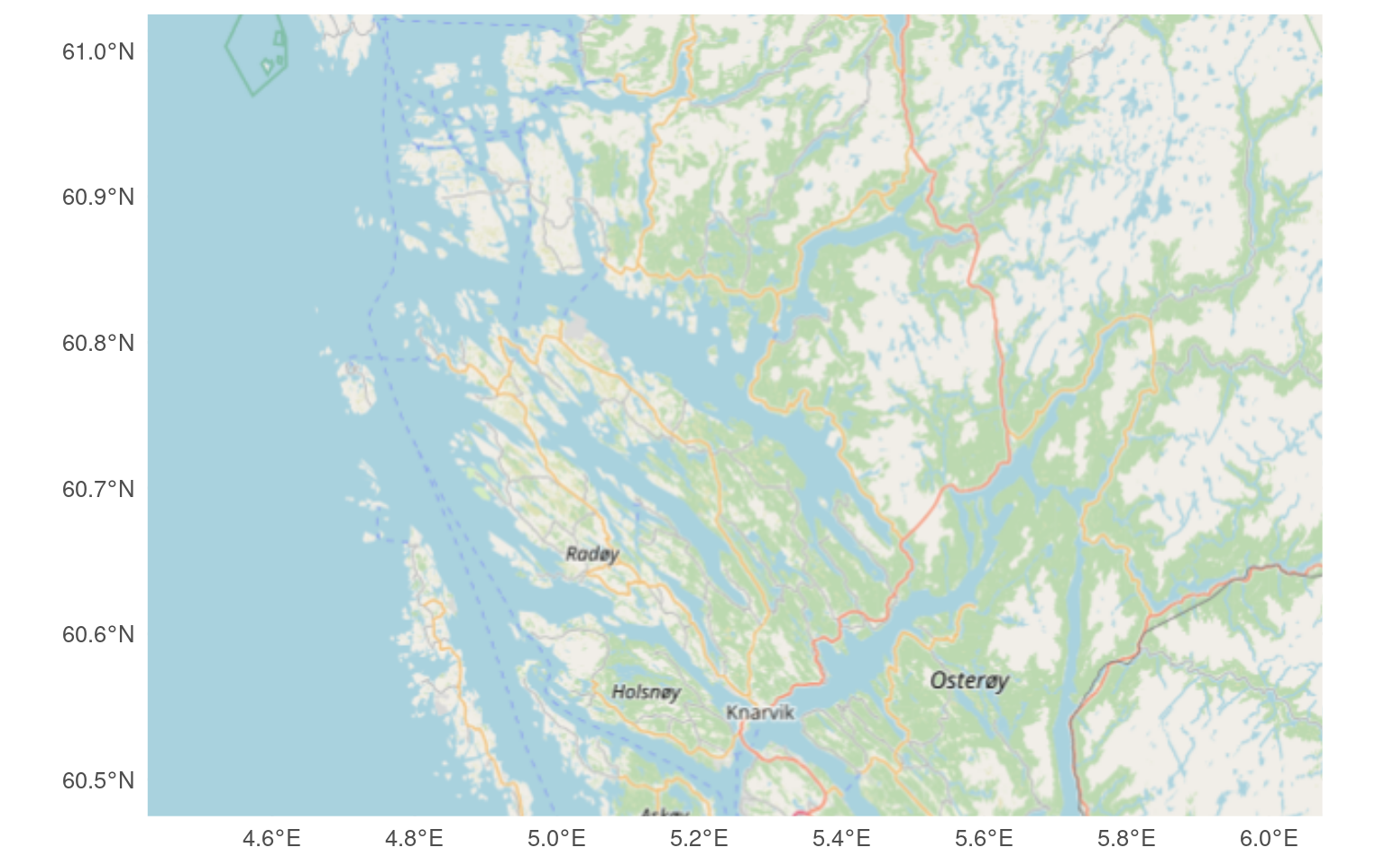
```{r}
#| label: anotation-map-tile
#| fig-width: 8
#| message: false
library(ggspatial)
ggplot() +
  annotation_map_tile(
    type = "osm",
    cachedir = "maps/",
    zoomin = -1
  ) + # sets the zoom level relative to the default
  coord_sf(
    xlim = c(4.5, 6),
    ylim = c(60.5, 61),
    crs = 4326
  ) # EPSG code for WGS84
```
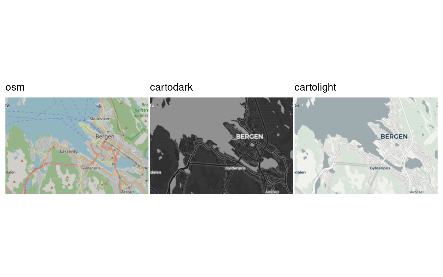
Several different types of maps are available (see `rosm::osm.types()`) and more can be added.
```{r}
#| label: map-providers
#| echo: false
#| fig-width: 8
#| message: false
#| fig-alt: maps of Bergen with different tiled backgrounds
# rosm::osm.types()
c("osm", "cartodark", "cartolight") |> # some need registration
map(\(osm_type) {
ggplot() +
annotation_map_tile(
type = osm_type,
cachedir = "maps/",
zoomin = -1
) +
coord_sf(
xlim = c(5.24, 5.36),
ylim = c(60.37, 60.41),
crs = 4326
) +
ggtitle(osm_type) +
theme(
axis.text = element_blank(),
axis.ticks = element_blank(),
title = element_text(size = 11),
plot.margin = margin(1, 1, 1, 1)
)
}) |>
patchwork::wrap_plots()
```
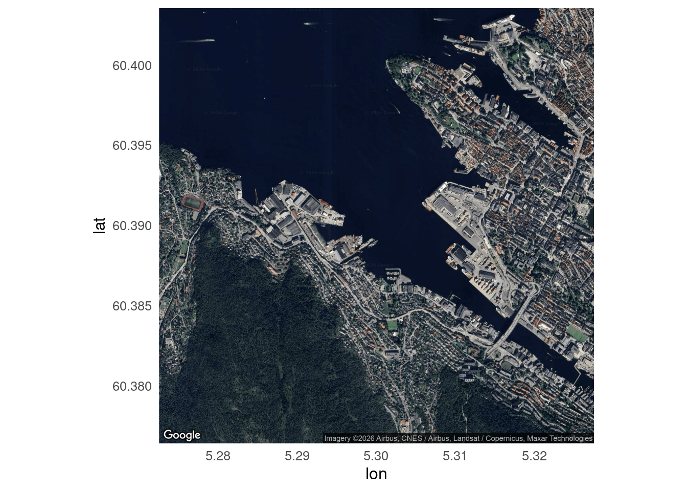
### `ggmap`
The `ggmap` package lets you use Google Maps, and and other similar maps as a basemap, including satellite imagery.
::: {.callout-tip collapse="true"}
## Using `ggmap`
`ggmap` can use maps and satellite image from Google, but you need to [register](https://mapsplatform.google.com/) for an API key.
You shouldn't be charged unless you make a lot of maps (thousands per month).
Then you can run this line in the console
```{r}
#| label: register-google
#| eval: false
# the write argument will save the key for you.
register_google(key = "[your key]", write = TRUE)
```
Your key is private.
Do not share it with anyone.
Do not include it your script or quarto document.
It could be expensive if someone else uses it.
Now you can use `ggmap`
```{r}
#| label: ggmap
#| message: false
#| fig-alt: Map of Bergen
library(ggmap)

bergen <- get_map(
  location = c(5.24, 60.37, 5.36, 60.41), # left/bottom/right/top
  maptype = "satellite"
)
ggmap(bergen)
```
This map made by `ggmap` is a `ggplot` object to which other geoms can be added.
:::
::: callout-note
## Exercise
Make a tiled map that shows your favourite holiday destination.
:::
## Adding data to the basemap
After deciding what type of base map to draw, we can add the data we want to show with the map.
This can be
- points, line, and polygons
- Shaded political units (a cloropleth map)
- A grid of values (raster)
### points/lines/polygons
Points lines and polygons can be added to the base map.
If the data are already a `sf` object they can be plotted with `geom_sf()`.
```{r}
#| label: second-sf
#| message: false
#| results: hide
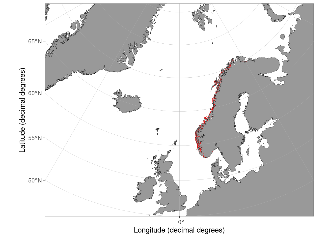
#| fig-alt: maps of aquaculture sites in Norway plotted with different packages
# aquaculture sites downloaded from Barentswatch.no/fiskinfo
aquaculture <- st_read("data/flate-ihht-akvakulturregisteret20220928.geojson")

# with rnaturalearth
ggplot() +
  geom_sf(data = europe) +
  geom_sf(data = aquaculture, colour = "red") +
  coord_sf(xlim = c(5, 30), ylim = c(55, 71))
# with ggOceanMaps

basemap(limits = c(-30, 30, 50, 80)) +
  geom_sf(data = aquaculture, colour = "red")
```
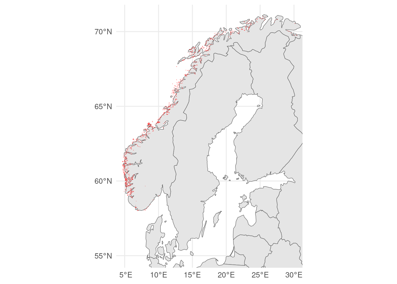
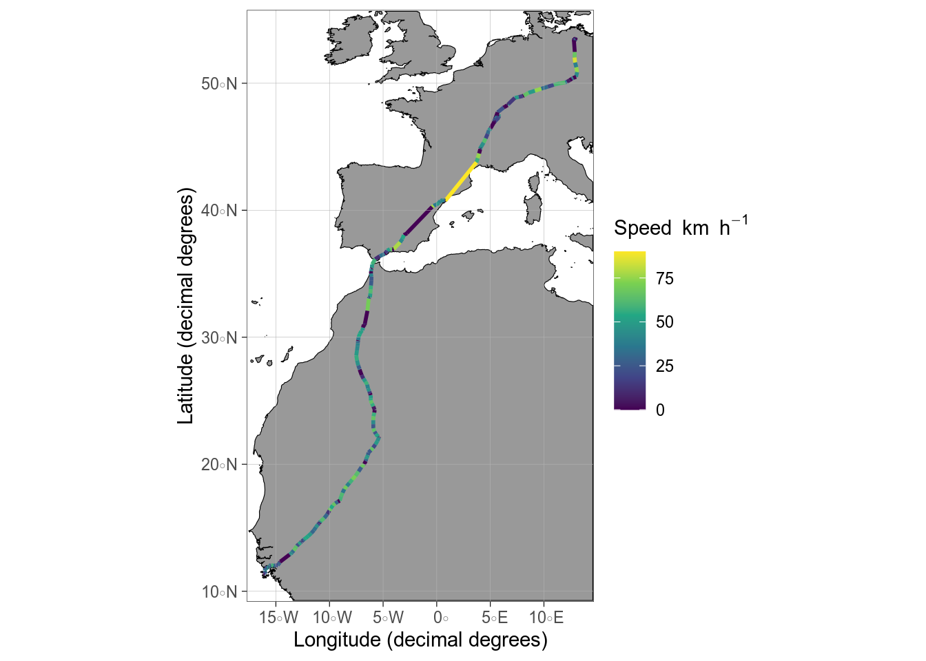
Alternatively, you can make/import a tibble with the geographic data and add them to the basemap with the relevant spatially aware geom from `ggspatial`.
So `geom_spatial_point()` rather than `geom_point()` and `geom_spatial_path()` rather than `geom_path()`.
```{r}
#| label: fig-geom-spatial-points
#| message: false
#| fig-cap: Flight speed of a migrating osprey
#| fig-alt: >
#| Maps showing flight speed of a migrating osprey from Germany to West Africa.
library(ggspatial)

# GPS tracking data of osprey. Data from
# https://datadryad.org/stash/dataset/doi:10.5061%2Fdryad.w6m905qt2
osprey <- read_delim("maps/osprey/06982.txt",
  locale = locale(decimal_mark = ",")
) |>
  janitor::clean_names()

# ggOceanMaps

basemap(data = osprey) +
  geom_spatial_path(aes(x = longitude_e, y = latitude_n, colour = speed),
    data = osprey, linewidth = 1
  ) +
  labs(colour = expression(Speed ~ km ~ h^{
    -1
  }))
```
`geom_spatial_point()` assumes that the data are latitude-longitude coordinates.
It they are UTM, you will need to use the `crs` argument with the correct [EPSG code](https://epsg.io/?q=UTM).
::: callout-tip
## geom_path() vs geom_line()
`geom_path()` draws a line from the first point in the dataset to the second and so on.
This is useful for plotting on maps with `geom_spatial_path()`.
`geom_line()` draws a line from the left-most point to the next left-most point in the dataset.
This is useful for plotting timeseries.
:::
::: callout-tip
## Degrees minutes and seconds
For latitude-longitude data, we recommend using decimal degrees (Bergen is at 60.3807°N, 5.3323°E).
But archived data can be in all sorts of unhelpful formats, such as degrees minutes and seconds (Bergen is at 60° 22' 50.52" N 5° 19' 56.28" E).
If you get data like this, you need to convert it to decimal degrees.
The `parzer` package can help (it is like `lubridate` for latitude-longitude data).
For example:
```{r}
#| label: parzer
parzer::parse_lat("60° 22' 50.52''N")
```
:::
::: callout-note
## Exercise
Otters (*Lutra lutra*) have re-established in Vestland.
File ExcelExport_7972978_Page_1a.xlsx, (from <https://artsobservasjoner.no>, edited to remove an invalid unicode character) shows observations of otters in Vestland.
Make a map of the observations.
Relevant columns are "East Coord", "North Coord".
The coordinates are UTM zone 33N, EPSG code 25833.
:::
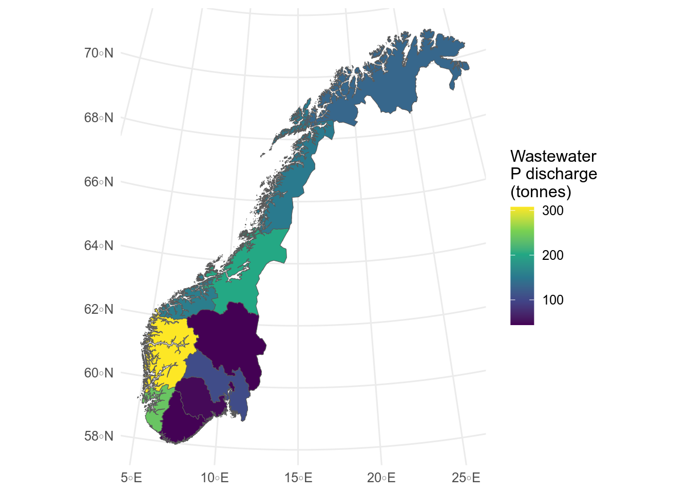
### Cloropleth maps
Cloropleth maps are useful for plotting data that have been aggregated to a geographic unit (kommune, fylke, country etc).
A `sf` object is a special type of data frame that we can `filter()`, `mutate()` or `left_join()` to other data frames.
We need a tibble with the data that we can join to the `sf` object with the geographic units.
Here, I use data on 2021 phosphorous discharge in municipal wastewater from [SSB](https://www.ssb.no/en/statbank/table/05280/) and join it by Fylkesnummer, and plot it by setting `fill` in the `aes`.
```{r}
#| label: fig-cloropleth
#| message: false
#| results: hide
#| fig-cap: Total phosphate discharge in municipal wastewater by fylke.
#| fig-alt: >
#| Cloropleth map of phosphate discharges by fylke.
#| Discharges are hightest in Vestland
p_discharge <- readxl::read_excel(
  path = "data/05280_20230421-012359.xlsx",
  skip = 4, n_max = 11
) |>
  janitor::clean_names() |>
  separate_wider_regex(
    cols = x1, # split fist column
    patterns = c(Fylkesnummer = "\\d{2}", " ", Fylkesnavn = ".*")
  ) # using regular expressions
# \\d{2} = 2 numbers
# " " = space
# ".*" = any number of any character, ie everything else

# join to fylker
fylker_2021 <- st_read("data/fylker2021.json") # older flyker map to match data
fylker_discharge <- fylker_2021 |>
  left_join(p_discharge, by = "Fylkesnummer")

ggplot(fylker_discharge) +
  geom_sf(aes(fill = total_discharge)) +
  labs(fill = "Wastewater\nP discharge\n(tonnes)")
```
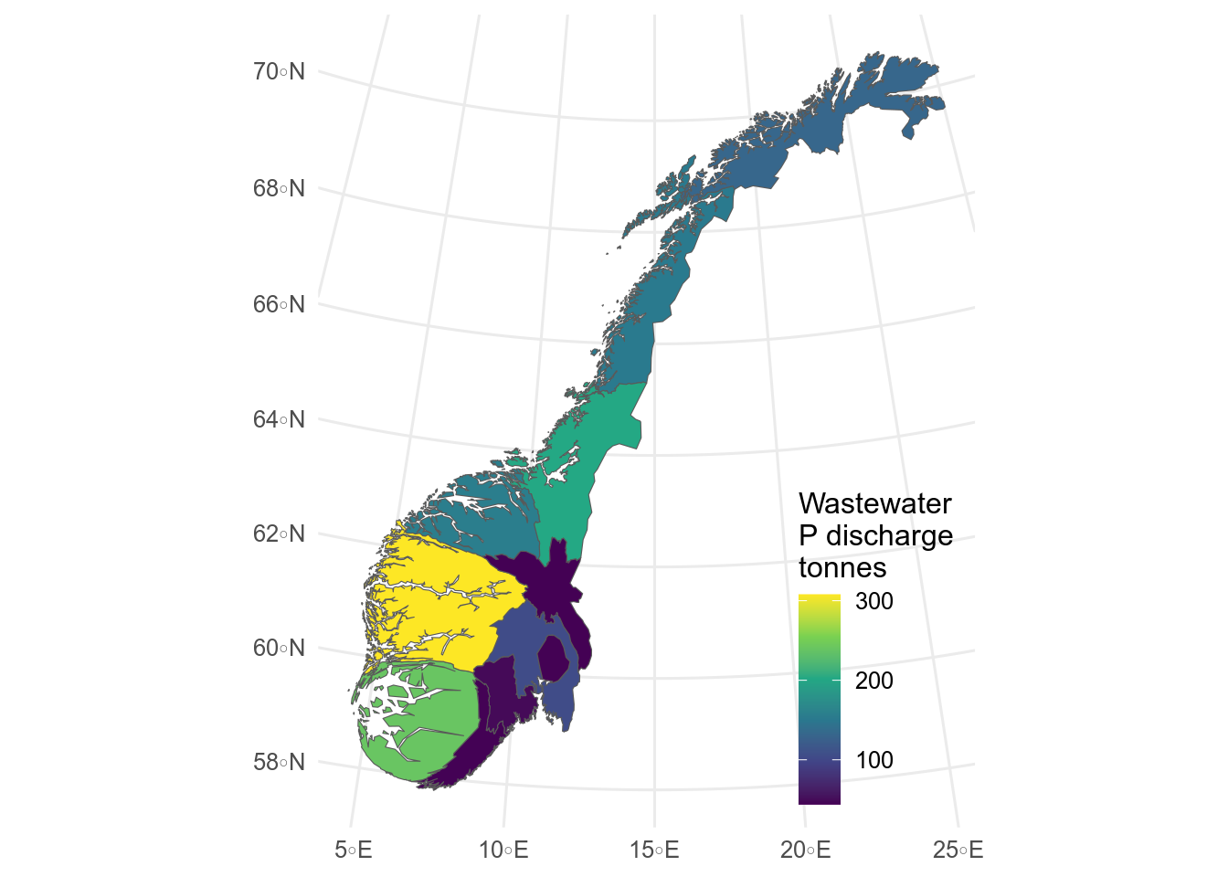
::: callout-tip
## Cartograms
Sometimes cloropleth maps can be misleading.
An alternative is to warp space so that the area of each region is proportional to the value.
This is a cartogram, which can be made with the `cartogram` package.
```{r}
#| label: fig-cartogram
#| message: false
#| fig-cap: >
#| Cartogram showing total phosphate discharge in municipal wastewater by fylke.
#| fig-alt: >
#| Cartogram showing total phosphate discharge in municipal wastewater by
#| fylke. Vestland is larger and Innlandet is smaller than in the normal map.
library(cartogram)

# simplify sf object for speed
fylker_discharge_sim <- sf::st_simplify(fylker_discharge, dTolerance = 1000)

# make cartogram
kart <- cartogram_cont(fylker_discharge_sim, weight = "total_discharge", itermax = 5)

# plot cartogram
ggplot(kart) +
  geom_sf(aes(fill = total_discharge)) +
  labs(fill = "Wastewater\nP discharge\ntonnes") +
  theme(
    legend.position.inside = c(.99, .01),
    legend.justification = c(1, 0)
  )
```
:::
::: callout-note
## Exercise
With `rnaturalearth` data, make a world map that shows the population (column pop_est) of each country.
:::
### Rasters
Rasters can be used to show maps of continuous data, for example, elevation or sea surface temperature, or model predictions.
Depending on the extent, you might not need a separate basemap.
### `terra`
The `terra` package can import raster images in several formats, including GeoTIFF.
::: callout-tip
## `terra` vs `raster` vs `stars` packages
The `terra` package is an update to the widely-used `raster` package.
It should be faster and easier to use.
`terra` can integrate with `ggplot2` with `tidyterra`.
`stars` is designed for spatio-temporal arrays.
There are some things it cannot do that `terra` can (and vice versa).
It has good integration with `sf` and `ggplot2`.
:::
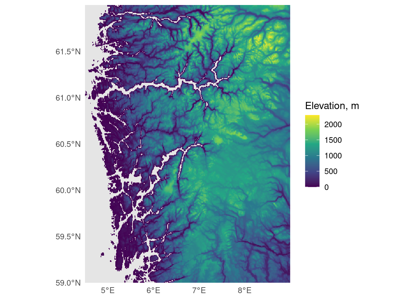
Rasters imported with `terra` are easy to plot with the base R `plot()` function, but if we want to use `ggplot()`, it is easiest to use a geom from the `tidyterra` package.
```{r}
#| label: terra
#| message: false
#| fig-alt: Raster map showing digital elevation model of vestland, cropped at sealevel.
library(terra)
library(tidyterra)

# import digital elevation model
# data from https://topotools.cr.usgs.gov/gmted_viewer/viewer.htm
norway_dem <- rast("data/50N000E_20101117_gmted_med300.tif")

# make coastline mask
coast_vector <- fylker |>
  # transfrom to crs of raster
  st_transform(crs = terra::crs(norway_dem)) |>
  # convert to spatVector
  vect()

# crop to vestland and rename the data layer
vestland_extent <- ext(4.5, 9, 59, 62)
vestland_dem <- crop(norway_dem, vestland_extent) |>
  mask(coast_vector) |>
  rename(Elevation = `50N000E_20101117_gmted_med300`)

# plot
ggplot() +
  geom_spatraster(data = vestland_dem) +
  scale_fill_viridis_c(na.value = "grey90") +
  scale_x_continuous(expand = c(0, 0)) +
  scale_y_continuous(expand = c(0, 0)) +
  labs(fill = "Elevation, m")
```
::: {.callout-tip collapse="true"}
## Raster map resources
- Low-resolution bathymetry - [GEBCO](https://www.gebco.net/data_and_products/gridded_bathymetry_data/) - some data also available through `ggOceanMaps`
- High-resolution bathymetry (50 m grid) (good for fjords - even higher resolution data is available for some regions) - from [mareano](https://mareano.no/en/maps-and-data) at [geonorge](https://kartkatalog.geonorge.no/metadata/kartverket/sjo-terrengmodeller-dtm-50/67a3a191-49cc-45bc-baf0-eaaf7c513549)
- 30 arc seconds (\~1 km) Digital elevation model - [GMTED2010](https://topotools.cr.usgs.gov/gmted_viewer/viewer.htm)
- High-resolution (1-50m LiDAR) digital elevation model - [Høydedata](https://hoydedata.no/LaserInnsyn2/)
- Climate normal data - [WorldClim](https://www.worldclim.org/data/worldclim21.html)
- Oceanographic conditions - [World Ocean Atlas](https://www.ncei.noaa.gov/products/world-ocean-atlas)
- Landsat - [NASA](https://search.earthdata.nasa.gov/)
:::
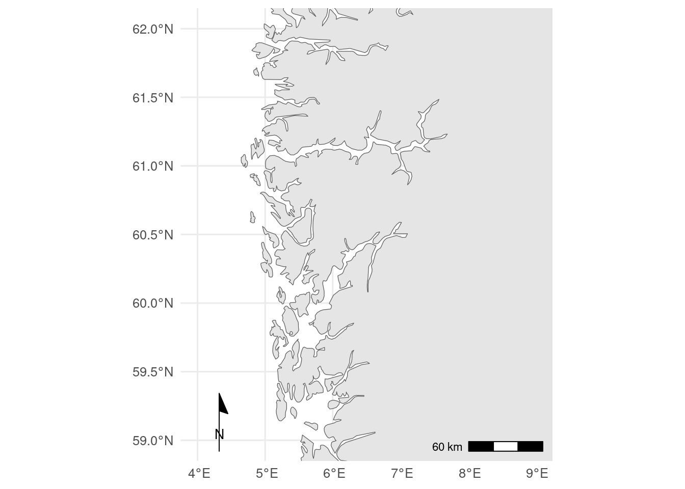
## Scalebars, north pointer etc
Scalebars and north pointers can be added with the `ggspatial` package or the `ggsn` package.
North points are not always necessary if the map has gridlines as these already indicate north.
A scalebar can be useful, especially for large scale map.
On small scale maps, they can be inaccurate as the scale varies.
```{r}
#| label: annotations
#| message: false
# with rnaturalearth
ggplot() +
  geom_sf(data = norway) +
  coord_sf(xlim = c(4, 9), ylim = c(59, 62)) +
  annotation_scale(location = "br") + # br = bottom right
  annotation_north_arrow(style = north_arrow_minimal)
```
## Hints for maps
**Keep it simple**.
Remove unnecessary features (do you really need to show the bathymetry?) and use appropriate scale data for the base map (too high resolution takes a long time to plot and can look worse).
Use **facets** as necessary (different species, different years etc).
If you need multiple colour scales, the `ggnewscale` package can help.
Use **inset maps** (@sec-combining-plots) to show your location in context.
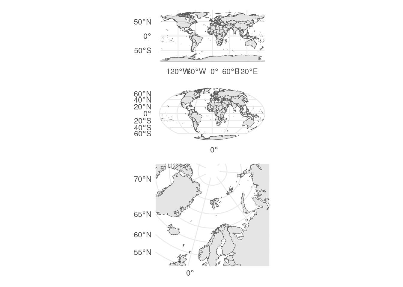
## Projections
The Earth is an oblate sphere and needs projecting to plot in two dimensions.
This inevitably leads to distortions, especially for maps with a large extent.
[Different projections](https://proj.org/operations/projections/index.html) have different properties and may be suitable for different purposes or regions.
`ggOceanMaps` can automatically select a projection based on the location, otherwise the map projection can be set using `coord_sf()`.
The [projection wizard](https://projectionwizard.org/#) can help choose a projection for a given area (copy the PROJ string).
```{r}
#| label: projections
#| results: hide
#| message: false
#| warning: false
world <- ne_countries(scale = "medium")

default <- ggplot(world) +
  geom_sf()

mollweide <- ggplot(world) + # Equal-area world map projection
  geom_sf() +
  coord_sf(crs = "+proj=moll") # projection specified with a 'proj' string

sf_use_s2(FALSE) # might need to turn spherical geometry off for some projections
polar_lambert <- world |>
  # !important - don't crop to tightly or crop lines will show in plot
  st_crop(y = c(xmin = -180, ymin = 50, xmax = 180, ymax = 90)) |>
  ggplot() + # Transverse cylindrical equal-area
  geom_sf() +
  # projection specified with a proj string
  coord_sf(
    crs = "+proj=laea +lon_0=14.4140625 +lat_0=90 +datum=WGS84 +units=m +no_defs",
    ylim = c(100000, -3500000), # xlim/ylim in units of projection
    xlim = c(-2000000, 2000000)
  ) # here in metres

default / mollweide / polar_lambert
```
::: callout-note
## Exercise
Change the projection of one of the small-scale maps you made previously.
:::
## Interactive maps
Interactive maps can be very useful on webpages and shiny apps, but less useful in theses and papers.
The [`leaflet`](https://rstudio.github.io/leaflet/) or [`mapgl`](https://walker-data.com/mapgl/index.html) packages can be used for fully interactive maps.
```{r}
#| label: fig-leaflet
#| fig-cap: >
#| leaflet map showing fish farms. You can zoom and pan the map, or click
#| to get the fish farm name.
#| fig-alt: Zoomable and panable map showing fish farm locations.
library(leaflet) # NB uses pipes |> not +

leaflet() |> # initialise map
  setView(lng = 5.3, lat = 60.4, zoom = 9) |> # set initial map area
  addTiles() |> # add background map
  addPolygons(data = aquaculture, popup = aquaculture$name) # add fish farms
```
It is possible to change the [background map](https://leaflet-extras.github.io/leaflet-providers/preview/) to one that is less cluttered or a satellite view.
::: callout-note
## Further reading
- [Spatial Data Science](https://r-spatial.org/book/)
- [Visualizing geospatial data](https://clauswilke.com/dataviz/geospatial-data.html)
:::
::: column-margin
### Contributors {.unlisted .unnumbered}
- Richard Telford
:::