21  Regression and ggplot

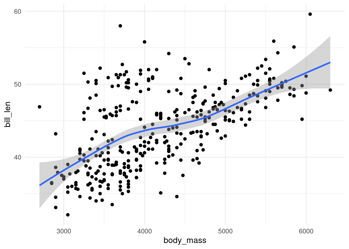
21.1 Regression lines with geom_smooth()

geom_smooth() adds a regression line to a plot. By default it uses a loess smooth when there are fewer than 1000 observations, and a GAM when there are more. The grey band around the regression line is the confidence interval. It can be turned off with se = FALSE, and changed from the default 95% with the level argument.

ggplot(penguins, aes(x = body_mass_g, y = bill_length_mm)) +
  geom_point() + 
  geom_smooth()

You can change they type of regression model used by geom_smooth() with the method argument. So to show a linear model, use method = "lm".

ggplot(penguins, aes(x = body_mass_g, y = bill_length_mm)) +
  geom_point() + 
  geom_smooth(method = "lm")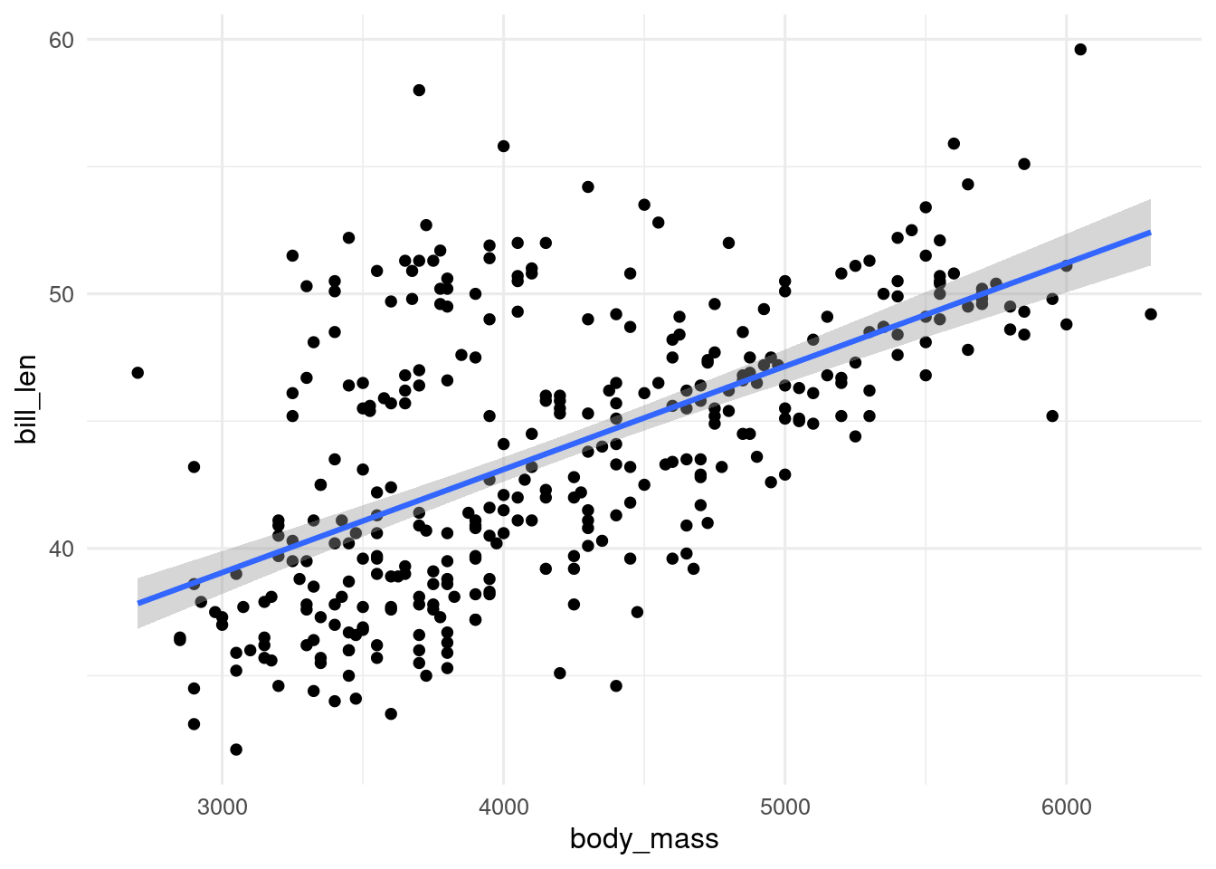

To show a glm, we need to method = "glm" and set the family in the method.args argument.

data(SWAP, package= "rioja")
swap_data <- bind_cols(pH = SWAP$pH, SWAP$spec)

ggplot(swap_data, aes(x = pH, y = sign(TA003A))) + # sign converts data to presence absence
  geom_jitter(width = 0, height = 0.1) +
  geom_smooth(
    method = "glm", 
    method.args = list(family = binomial)) +
  scale_y_continuous(breaks = c(0, 1)) +
  labs(y = expression(italic(Tabellaria~binalis)))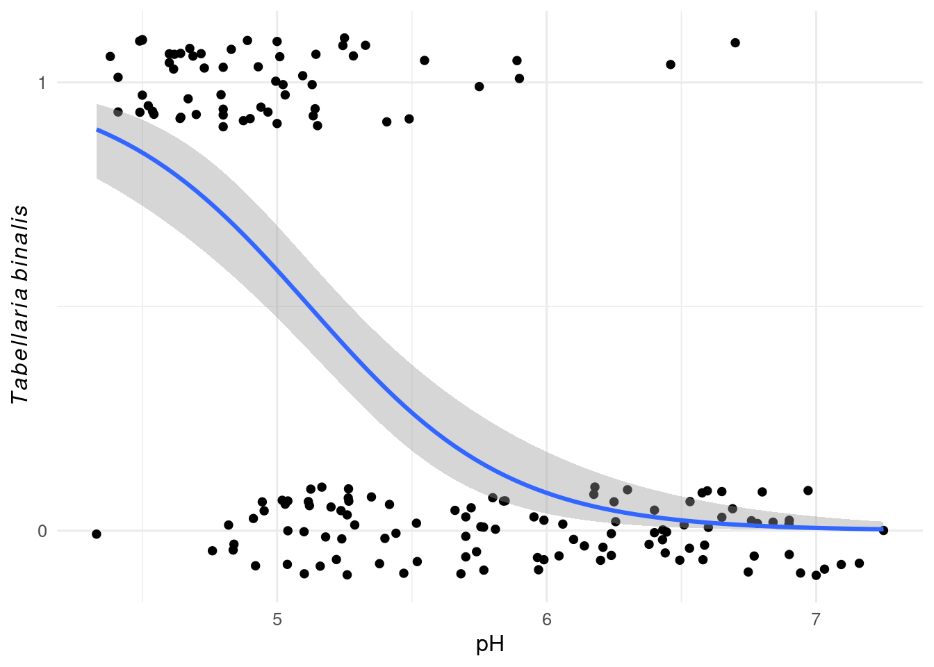 

21.2 Manual plotting of a linear model

We can also fit a regression model and make predictions. This is most useful for more complex models. For example, if we want to fit a model for the relationship between penguin body mass and bill length with species as a second predictor, we can only do it this way.

First fit the model

mod <- lm(bill_length_mm ~ body_mass_g + species, 
          data = penguins)

Now we need to make predictions. We could do this with predict(), but it is often easier to use augment() from the broom package as it takes care of missing values better.

#preds <- predict(mod, interval = "confidence", conf.level = 0.95)

# augment with a lm model
preds <- broom::augment(mod, interval = "confidence",  conf.level = 0.95)

Now we can plot them, using geom_ribbon() and geom_line() to recreate what geom_smooth() produces.

ggplot(penguins, aes(x = body_mass_g, y = bill_length_mm, fill = species)) +
  geom_point(aes(colour = species)) +
  geom_ribbon(aes(ymin = .lower, ymax = .upper), data = preds, alpha = 0.3) +
  geom_line(aes(y = .fitted, colour = species), data = preds) + 
  labs(x = "Body mass g", y = "Bill length mm")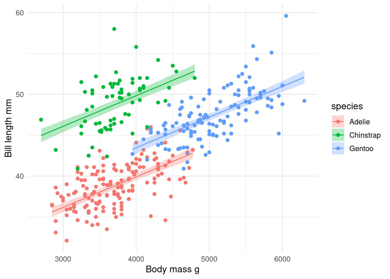

21.3 Manual plotting of generalised linear models

With a generalised linear model, it is a little more complex as we can get the predictions on the response scale or the transformed link scale. If we want confidence intervals, we need to calculate them on the link scale and then transform them back to the response scale.

With a poisson model, we can transform the predictions from the link scale to the response scale with the exponential function exp().

With a binomial model, we need to reverse the logit function. The easiest way to do this is with plogis().

mod_glm <- glm(sign(TA003A) ~ pH, data = swap_data, family = binomial)

preds_glm <- broom::augment(mod_glm, type.predict = "link", se_fit = TRUE) |> 
  mutate(
    fitted = plogis(.fitted), 
    lower = plogis(.fitted + .se.fit * 1.96),
    upper = plogis(.fitted - .se.fit * 1.96),
  )

Now we can plot the predictions.

ggplot(swap_data, aes(x = pH, y = sign(TA003A))) + # sign converts data to presence absence
  geom_jitter(width = 0, height = 0.1) +
  geom_ribbon(aes(ymax = upper, ymin = lower, y = NULL),
              data = preds_glm, alpha = 0.3) +
  geom_line(aes(y = fitted),
              data = preds_glm) +
  scale_y_continuous(breaks = c(0, 1)) +
  labs(y = expression(italic(Tabellaria~binalis)))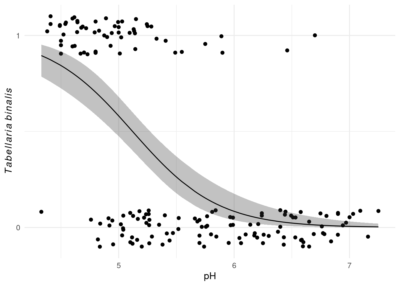 

21.4 Mixed effect models

Comming soon …

Contributors

• Richard Telford