23  Combining plots

We often need to combine plots to make a multipart figure in a manuscript or thesis.

First, check you actually need to combine plots and cannot use facets instead. Typically, use facets if the x-axis variable is the same for all plots and the plots use the same geoms.

Plots can be combined using the patchwork package.

library(patchwork)

Start by making some plots

p1 <- ggplot(penguins, aes(x = species, y = bill_len)) +
  geom_boxplot()
p2 <- ggplot(penguins, aes(x = body_mass, y = bill_len, colour = species)) +
  geom_point()
p3 <- ggplot(penguins, aes(x = body_mass, y = bill_len, colour = species)) +
  geom_point() +
  facet_wrap(facets = vars(species))
p4 <- ggplot(penguins, aes(x = island, fill = species)) +
  geom_bar()

The simplest way to use patchwork is to + to combine the plots. patchwork will try to make the combined figure square.

p1 + p2 + p3 + p4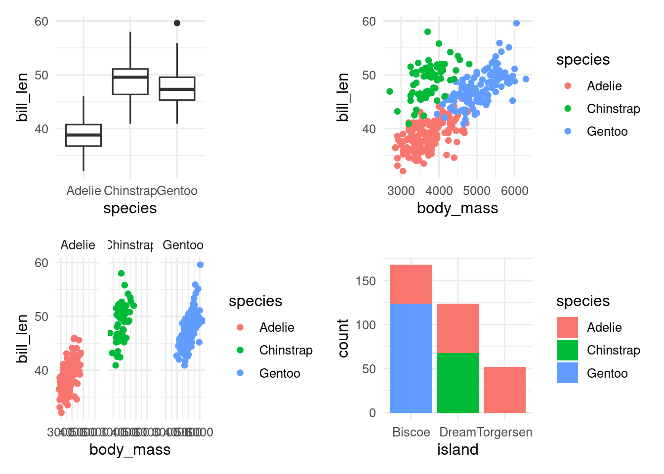

With | (side by side) \ (over under), you can have more control.

(p1 | p2 | p4) / p3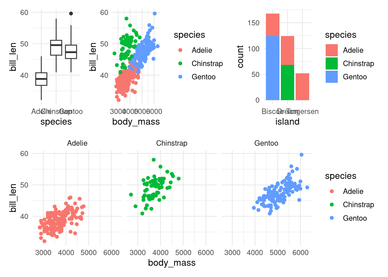

plot_layout gives you control over the relative size of the plot and whether the legends should be combined if possible.

(p1 | p2 | p4) / p3 +
  plot_layout(heights = c(2, 1), guides = "collect")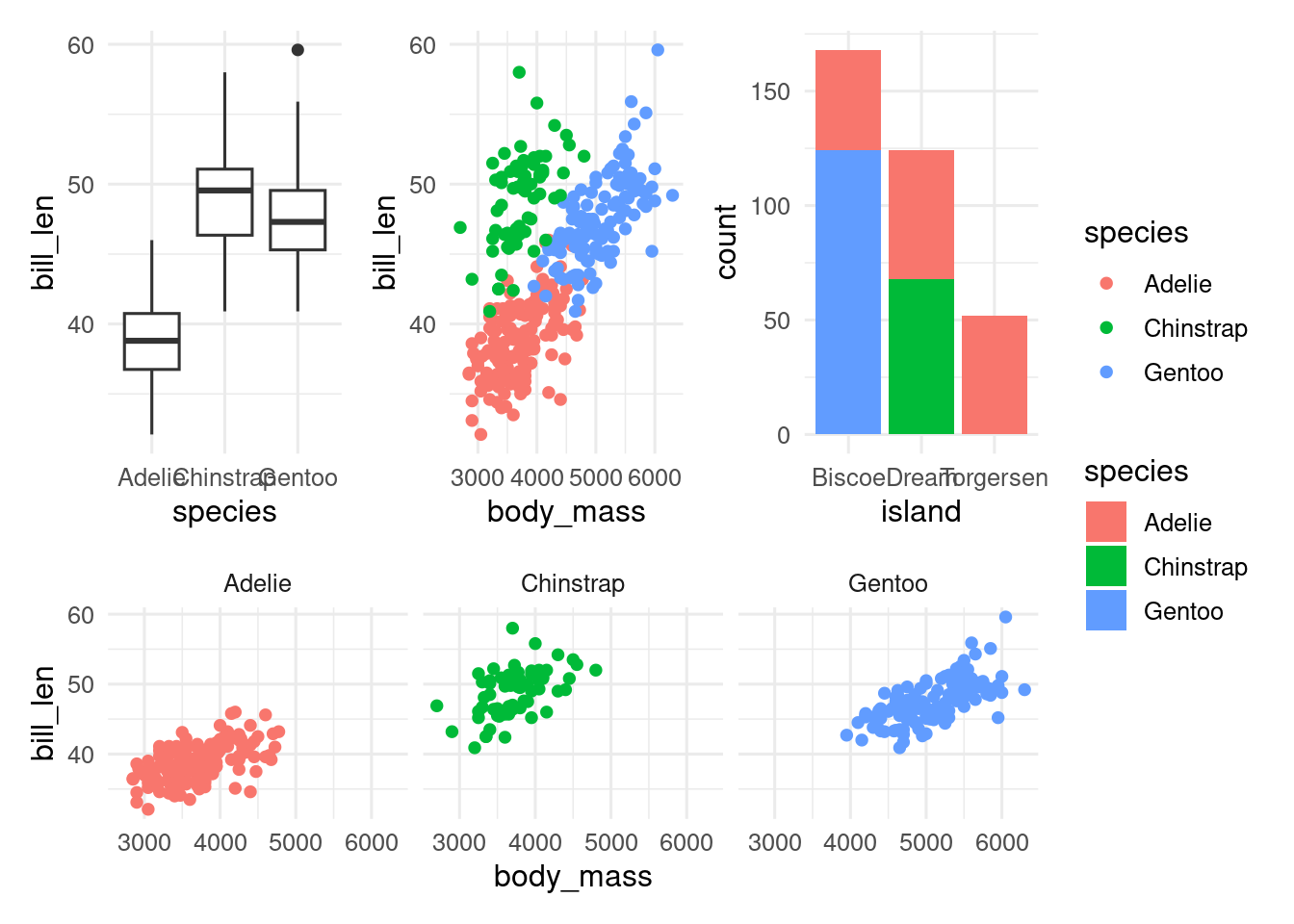

If you want to change all the plots in the combined figure, you can add a ggplot2 function with &.

(p1 | p2 | p4) / p3 +
  plot_layout(heights = c(2, 1), guides = "collect") &
  theme(panel.grid = element_blank())

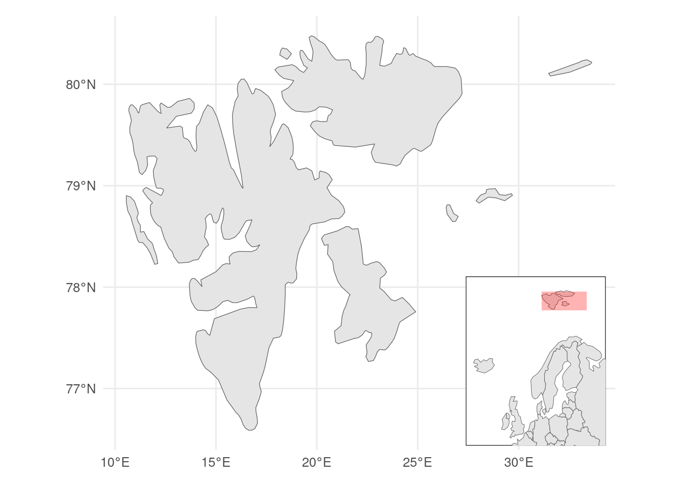
You can also overlay figures, which might be useful to show an inset map.

library(rnaturalearth)
library(sf)

# map data inset
europe <- ne_countries(scale = 110, continent = "Europe", returnclass = "sf")

# map data main map
svalbard <- ne_countries(scale = 50, country = "Norway", returnclass = "sf") |>
  st_crop(c(xmin = 0, xmax = 34, ymin = 76, ymax = 81))

# bounding box main map
bb <- svalbard |>
  st_bbox()

# inset map
euro_map <- ggplot() +
  geom_sf(data = europe) +
  # annotate bounding box
  annotate(
    geom = "rect",
    xmin = bb$xmin, xmax = bb$xmax, ymin = bb$ymin, ymax = bb$ymax,
    fill = "red", alpha = 0.3
  ) +
  coord_sf(xlim = c(-25, 40), y = c(50, 82)) +
  ggthemes::theme_map() +
  theme(
    # give white background and black border
    panel.background = element_rect(fill = "white", colour = "black"),
    plot.margin = margin() # remove margins
  )

# main map
svalbard_map <- ggplot() +
  geom_sf(data = svalbard)

# combined map
svalbard_map +
  inset_element(euro_map,
    left = 0.7,
    right = 0.99,
    top = 0.4,
    bottom = 0.01
  )

NoteFurther reading

patchwork package

Contributors

• Richard Telford