13 Tidying data with `tidyr`

13.1 Tidy data

Before you can start analysing or plotting data, you often need to tidy it. Tidy data is a standardised way to structure a dataset which makes it much easier to process, analyse and plot the data. Functions in the tidyr and dplyr packages, both part of tidyverse, can be very useful for tidying data.

library(tidyr)

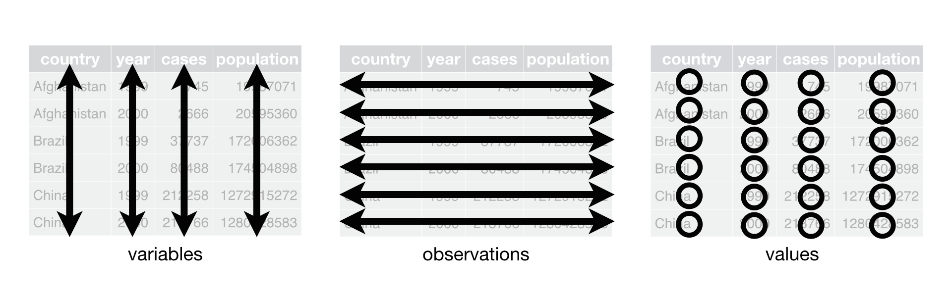
Tidy data is a standard, consistent way to organize tabular data. Briefly, tidy data follows a short series of rules:

each variable in the data set is presented in a specific column,
each observation in the data set is presented in a specific row,
each cell at the intersection of a row and a column contains a single value.

The following figure illustrates these rules.

Schematic diagram showing that variables should be in columns, observations in rows and each cell should contain a single value — In a tidy dataset, variables are in columns, observations are in rows, and values are in cells. — Source: R for Data Science

The dataset presented in Table 11.1 respects all three rules, and is thus a tidy dataset.

On the contrary, the following dataset is not tidy:

Date	17.06.2016	21.06.2016	23.06.2016	26.06.2016	27.06.2016	28.06.2016	29.06.2016	30.06.2016	02.07.2016	04.07.2016	05.07.2016	06.07.2016	08.07.2016	10.07.2016	11.07.2016	13.07.2016	15.07.2016	17.07.2016	19.07.2016	21.07.2016	23.07.2016	24.07.2016	26.07.2016	28.07.2016	30.07.2016	02.08.2016	04.08.2016	06.08.2016	11.08.2016
Time	10:00	11:00	11:00	13:00	13:00	09:33	13:00	15:00	09:00	09:15	09:30	09:15	09:15	09:15	09:15	09:30	10:00	13:00	17:30	10	10:00	09:30	09:30	09:30	09:15	09:30	15:00	11:00	15:00
Weather	Sunny_PartlyCloudy	Cloudy_Fog	Cloudy_Sunny	Cloudy_Rainy_Windy_Fog	Cloudy_Windy_Rainy	Windy_Rainy_MostlyCloudy	Windy_Sunny_Cloudy	Windy_Cloudy	Windy_Cloudy	Cloudy_Sunny	Cloudy_Sunny	Cloudy_Fog_Rainy	Sunny_PartlyCloudy	Cloudy_Rainy	Cloudy	Cloudy_Sunny	Cloudy	Cloudy_Rainy	Cloudy_Rainy	Cloudy_Sunny	Sunny_Cloudy	Cloudy_Sunny	Cloudy_Rainy	Cloudy_Rainy	Cloudy_Rainy	Cloudy_Rainy	Cloudy_Rainy	Cloudy_Rainyn	Cloudy_Snowy_Sunny
Observer	LV_AH	LV	LV	LV	LV_SB	LV_SB	LV_SB	LV	LV_SB	SB_LV	SB_LV	LV_SB	LV_SB	LV_SB	LV	LV	LV_SB_AH	SB_LV	SB_LV	SB_LV	SB_LV	LV	LV	LV	LV	LV	LV	LV	LV
E01a	0	NA	0	0	0	0	1	1	2	2	3	3	6	8	8	11	13	10	9	7	3	6	3	3	1	1	1	2	1
E01b	0	NA	0	0	1	1	1	1	1	1	1	1	3	3	3	8	19	23	26	24	16	16	8	5	2	3	4	3	2
E01c	0	NA	0	0	0	0	0	0	0	0	0	0	0	0	1	5	9	12	10	7	4	3	3	3	2	2	0	1	1
E01d	0	NA	0	0	0	0	0	0	0	0	0	0	1	1	1	2	4	3	2	4	1	1	1	2	2	1	1	1	0
E01e	0	NA	0	0	0	0	0	0	0	0	0	0	0	0	0	1	4	4	4	5	4	3	1	0	0	0	0	0	0

Indeed, at least one of the rules is broken since columns display data matching several variables (Date, time, Weather, etc).

Importing data from a file containing tidy data is a great way to start your work, but it is not a prerequisite to data import. As long as your data is tabular, you will be able to import it in R, and tidy it later.

The process of tidying data is to convert the data you have to data that meets this standard.

13.2 Multiple values in a cell

If a cell contains multiple values, we need to separate to tidy the data. We can separate the values into multiple columns with tidyr::separate_wider_delim(). For example, in this small dataset, site code and plot number have been combined into one column separated by a hyphen.

dat <- tribble(~id, ~value,
       "A-1", 1,
       "A-2", 2,
       "B-1", 3)

dat

# A tibble: 3 × 2
  id    value
  <chr> <dbl>
1 A-1       1
2 A-2       2
3 B-1       3

We can use separate_wider_delim() to split site and plot into separate columns. The delimited is set by the delim argument.

dat |> 
  separate_wider_delim(cols = id, delim = "-", names = c("site", "plot"))

# A tibble: 3 × 3
  site  plot  value
  <chr> <chr> <dbl>
1 A     1         1
2 A     2         2
3 B     1         3

Related function, separate_wider_regex(), which uses regular expressions to split the column, can be more flexible.

If there are multiple measurements of the same type in a single cell, then tidyr::separate_longer_delim() can be useful to separate the data into multiple rows.

13.3 Reshaping data - wide to long

It is very common to need to reshape data to make it tidy. This can be done with the pivot_* functions.

Wide data to long data with `pivot_longer()` and `pivot_wider()` .

These are some Bergen climate data from Wikipedia (NB for demonstration only wikipedia is not a good source of climate data - use seklima for Norwegian data).

Rows: 4 Columns: 13
── Column specification ────────────────────────────────────────────────────────
Delimiter: "\t"
chr  (1): Måned
dbl (12): Jan, Feb, Mar, Apr, Mai, Jun, Jul, Aug, Sep, Okt, Nov, Des

ℹ Use `spec()` to retrieve the full column specification for this data.
ℹ Specify the column types or set `show_col_types = FALSE` to quiet this message.

# A tibble: 4 × 13
  Måned    Jan   Feb   Mar   Apr   Mai   Jun   Jul   Aug   Sep   Okt   Nov   Des
  <chr>  <dbl> <dbl> <dbl> <dbl> <dbl> <dbl> <dbl> <dbl> <dbl> <dbl> <dbl> <dbl>
1 Norma…   3.6   4     5.9   9.1  14    16.8  17.6  17.4  14.2  11.2   6.9   4.7
2 Døgnm…   1.7   1.7   3.3   5.8  10.4  13.1  14.2  14.2  11.5   8.8   4.8   2.7
3 Norma…  -0.4  -0.5   0.9   3     7.2  10.2  11.5  11.6   9.1   6.6   2.8   0.6
4 Nedbø… 190   152   170   114   106   132   148   190   283   271   259   235

This might be a nice way to present the data but it is not tidy data: each row is not an observation; each column is not a variable.

We can use pivot_longer() to reshape the data. The months, selected by the cols argument in the column names (see Section 14.2.1 for more on the syntax used here) will become a new variable with a name set by the names_to, and the data values get put into a column named by the values_to argument.

bergen_klima_long <- bergen_klima |> 
  pivot_longer(cols = Jan:Des, names_to = "Month", values_to = "value")
bergen_klima_long

# A tibble: 48 × 3
  Måned                 Month value
  <chr>                 <chr> <dbl>
1 Normal maks. temp. °C Jan     3.6
2 Normal maks. temp. °C Feb     4  
3 Normal maks. temp. °C Mar     5.9
# ℹ 45 more rows

The data are now tidier, but it would probably be more useful to reshape the data again, and have a column for each climate variable. We can do this pivot_wider().

13.4 Reshaping data - long to wide

We can tell pivot_wider() which column contains what will become the column names and the data with the names_from and values_from, respectively.

bergen_klima_wider <- bergen_klima_long |> 
  pivot_wider(names_from = "Måned", values_from = "value")

bergen_klima_wider

# A tibble: 12 × 5
   Month `Normal maks. temp. °C` `Døgnmiddeltemp. °C` `Normal min. temp. °C`
   <chr>                   <dbl>                <dbl>                  <dbl>
 1 Jan                       3.6                  1.7                   -0.4
 2 Feb                       4                    1.7                   -0.5
 3 Mar                       5.9                  3.3                    0.9
 4 Apr                       9.1                  5.8                    3  
 5 Mai                      14                   10.4                    7.2
 6 Jun                      16.8                 13.1                   10.2
 7 Jul                      17.6                 14.2                   11.5
 8 Aug                      17.4                 14.2                   11.6
 9 Sep                      14.2                 11.5                    9.1
10 Okt                      11.2                  8.8                    6.6
11 Nov                       6.9                  4.8                    2.8
12 Des                       4.7                  2.7                    0.6
# ℹ 1 more variable: `Nedbør (mm)` <dbl>

The data are now in a convenient format for plotting or analysis.

Exercise

With the Mt Gonga data downloaded previously, pivot the data so that the height data (H1-H10) are in one column.

Hint

pivot_longer

Contributors

Richard Telford